mages' blog

Transforming data sets with R is usually the starting point of my data analysis work. Here is a scenario which comes up from time to time: transform subsets of a data frame, based on context given in one or a combination of columns.

As an example I use a data set which shows sales figures by product for a number of years:

df <- data.frame(Product=gl(3,10,labels=c("A","B", "C")), 
                 Year=factor(rep(2002:2011,3)), 
                 Sales=1:30)
head(df)
##   Product Year Sales
## 1       A 2002     1
## 2       A 2003     2
## 3       A 2004     3
## 4       A 2005     4
## 5       A 2006     5
## 6       A 2007     6

I am interested in absolute and relative sales developments by product over time. Hence, I would like to add a column to my data frame that shows the sales figures divided by the total sum of sales in each year, so I can create a chart which looks like this:
There are lots of ways of doing this transformation in R. Here are three approaches using:

• base R with by,
• ddply of the plyr package,
• data.table of the package with the same name.

by

The idea here is to use by to split the data for each year and to apply the transform function to each subset to calculate the share of sales for each product with the following function: fn <- function(x) x/sum(x). Having defined the function fn I can apply it in a by statement, and as its output will be a list, I wrap it into a do.call command to row-bind (rbind) the list elements:

R1 <- do.call("rbind", as.list(
  by(df, df["Year"], transform, Share=fn(Sales))
))

head(R1)
##         Product Year Sales      Share
## 2002.1        A 2002     1 0.03030303
## 2002.11       B 2002    11 0.33333333
## 2002.21       C 2002    21 0.63636364
## 2003.2        A 2003     2 0.05555556
## 2003.12       B 2003    12 0.33333333
## 2003.22       C 2003    22 0.61111111

ddply

Hadely's plyr package provides an elegant wrapper for this job with the ddply function. Again I use the transform function with my self defined fn function:

library(plyr)
R2 <- ddply(df, "Year", transform, Share=fn(Sales))

head(R2)
##   Product Year Sales      Share
## 1       A 2002     1 0.03030303
## 2       B 2002    11 0.33333333
## 3       C 2002    21 0.63636364
## 4       A 2003     2 0.05555556
## 5       B 2003    12 0.33333333
## 6       C 2003    22 0.61111111

data.table

With data.table I have to do a little bit more legwork, in particular I have to think about the indices I need to use. Yet, it is still straight forward:

library(data.table)
## Convert df into a data.table
dt <- data.table(df) 
## Set Year as a key
setkey(dt, "Year") 
## Calculate the sum of sales per year(=key(dt))
X <- dt[, list(SUM=sum(Sales)), by=key(dt)] 
## Join X and dt, both have the same key and
## add the share of sales as an additional column
R3 <- dt[X, list(Sales, Product, Share=Sales/SUM)]

head(R3)
##      Year Sales Product      Share
## [1,] 2002     1       A 0.03030303
## [2,] 2002    11       B 0.33333333
## [3,] 2002    21       C 0.63636364
## [4,] 2003     2       A 0.05555556
## [5,] 2003    12       B 0.33333333
## [6,] 2003    22       C 0.61111111

Although data.table may look cumbersome compared to ddply and by, I will show below that it is actually a lot faster than the two other approaches.

Plotting the results

With any of the three outputs I can create the chart from above with latticeExtra:

library(latticeExtra)
asTheEconomist(
 xyplot(Sales + Share ~ Year, groups=Product, 
  data=R3, t="b", 
  scales=list(relation="free",x=list(rot=45)), 
  auto.key=list(space="top", column=3),
  main="Product information")
)

Comparing performance of by, ddply and data.table

Let me move on to a more real life example with 100 companies, each with 20 products and a 10 year history:

set.seed(1)
df <- data.frame(Company=rep(paste("Company", 1:100),200),
                 Product=gl(20,100,labels=LETTERS[1:20]), 
                 Year=sort(rep(2002:2011,2000)), 
                 Sales=rnorm(20000, 100,10))

I use the same three approaches to calculate the share of sales by product for each year and company, but this time I will measure the execution time on my old iBook G4, running R-2.15.0:

r1 <- system.time(
 R1 <- do.call("rbind", as.list(
   by(df, df[c("Year", "Company")], 
      transform, Share=fn(Sales))
 ))
)

r2 <- system.time(
 R2 <- ddply(df, c("Company", "Year"), 
             transform, Share=fn(Sales))
)

r3 <- system.time({
 dt <- data.table(df)
 setkey(dt, "Year", "Company")
 X <- dt[, list(SUM=sum(Sales)), by=key(dt)]
 R3 <- dt[X, list(Company, Sales, Product, Share=Sales/SUM)]
})

And here are the results:

r1 # by
##  user  system elapsed 
## 13.690   4.178  42.118 
r2 # ddply 
##  user  system elapsed 
## 18.215   6.873  53.061
r3 # data.table 
##  user  system elapsed 
## 0.171   0.036   0.442

It is quite astonishing to see the speed of data.table in comparison to by and ddply, but maybe it shouldn't be surprise that the elegance of ddply comes with a price as well.

Addition (13 June 2012): See also Matt's comments below. I completely missed ave from base R, which is rather simple and quick as well. Additionally his link to a stackoverflow discussion provides further examples and benchmarks.

Finally my session info:

> sessionInfo() # iBook G4 800 MHZ, 640 MB RAM
R version 2.15.0 Patched (2012-06-03 r59505)
Platform: powerpc-apple-darwin8.11.0 (32-bit)

locale:
[1] C

attached base packages:
[1] stats     graphics  grDevices utils     datasets  methods   base     

other attached packages:
[1] latticeExtra_0.6-19 lattice_0.20-6      RColorBrewer_1.0-5 
[4] data.table_1.8.0    plyr_1.7.1         

loaded via a namespace (and not attached):
[1] grid_2.15.0

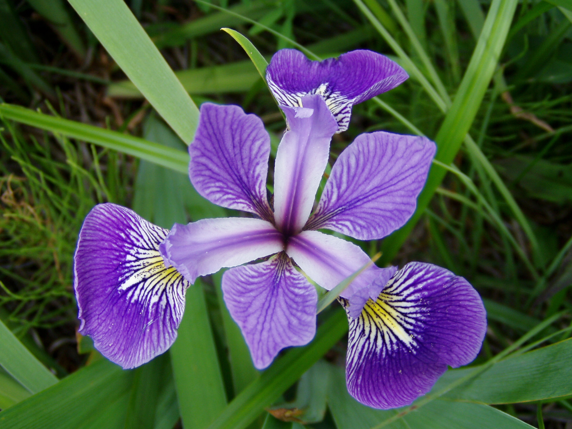Iris versicolor  By Danielle Langlois License: CC-BY-SA

R is a language, as Luis Apiolaza pointed out in his recent post. This is absolutely true, and learning a programming language is not much different from learning a foreign language. It takes time and a lot of practice to be proficient in it. I started using R when I moved to the UK and I wonder, if I have a better understanding of English or R by now.

Languages are full of surprises, in particular for non-native speakers. The other day I learned that there is courtesy and curtsey. Both words sounded very similar to me, but of course created some laughter when I mixed them up in an email.

With languages you can get into habits of using certain words and phrases, but sometimes you see or hear something, which shakes you up again. So did the following two lines in R with me:

f <- function(x) x^2
sapply(1:10, f)
[1]   1   4   9  16  25  36  49  64  81 100

It reminded me of the phrase that everything is a list in R. It showed me again how easily a for loop can be turned into a statement using the apply family of functions and how little I know about all the subtleties of R. I remember how happy I felt, when I finally understood the by function in R. I started to use it all the time, closing my eyes on aggregate and the apply functions family. Here is an example where I calculate the means of the various measurements by species of the famous iris data set using by.

by

do.call("rbind", as.list(
  by(iris, list(Species=iris$Species), function(x){
    y <- subset(x, select= -Species)
    apply(y, 2, mean)
  }
)))

           Sepal.Length Sepal.Width Petal.Length Petal.Width
setosa            5.006       3.428        1.462       0.246
versicolor        5.936       2.770        4.260       1.326
virginica         6.588       2.974        5.552       2.026

Now let's find alternative ways of expressing ourselves, using other words/functions of the R language, such as aggregate, apply, sapply, tapply, data.table, ddply, sqldf, and summaryBy.

aggregate

The aggregate function splits the data into subsets and computes summary statistics for each of them. The output of aggregate is a data.frame, including a column for species.

iris.x <- subset(iris, select= -Species)
iris.s <- subset(iris, select= Species)
aggregate(iris.x, iris.s, mean)

     Species Sepal.Length Sepal.Width Petal.Length Petal.Width
1     setosa        5.006       3.428        1.462       0.246
2 versicolor        5.936       2.770        4.260       1.326
3  virginica        6.588       2.974        5.552       2.026

Addition: As John Christie points out in the comments, aggregate has also a formula interface, which simplifies the call to:

aggregate( . ~ Species, iris, mean)

apply and tapply

The combination of tapply and apply achieves a similar result, but this time the output is a matrix and hence I lose the column with species. The species are now the row names.

apply(iris.x, 2, function(x) tapply(x, iris.s, mean))

           Sepal.Length Sepal.Width Petal.Length Petal.Width
setosa            5.006       3.428        1.462       0.246
versicolor        5.936       2.770        4.260       1.326
virginica         6.588       2.974        5.552       2.026

split and apply

Here I split the data first into subsets for each of the species and calculate then the mean for each column in the subset. The output is a matrix again, but transposed.

sapply(split(iris.x, iris.s), function(x) apply(x, 2, mean))

             setosa versicolor virginica
Sepal.Length  5.006      5.936     6.588
Sepal.Width   3.428      2.770     2.974
Petal.Length  1.462      4.260     5.552
Petal.Width   0.246      1.326     2.026

ddply

Hadley Wickham's plyr package provides tools for splitting, applying and combining data. The function ddply is similar to the by function, but it returns a data.frame instead of a by list and maintains the column for the species.

library(plyr)
ddply(iris, "Species", function(x){
    y <- subset(x, select= -Species)
    apply(y, 2, mean)
  })

     Species Sepal.Length Sepal.Width Petal.Length Petal.Width
1     setosa        5.006       3.428        1.462       0.246
2 versicolor        5.936       2.770        4.260       1.326
3  virginica        6.588       2.974        5.552       2.026

Addition: Sean mentions in the comments an alternative, using the colMeans function, while Andrew reminds us of the reshape package with its functions melt and cast.

ddply(iris, "Species", function(x) colMeans(subset(x, select= -Species)))
## or
ddply(iris, "Species", colwise(mean)) 
## same output as above
library(reshape)
cast(melt(iris, id.vars='Species'),formula=Species ~ variable,mean)
## same output as above

summaryBy

The summaryBy function of the doBy package by Søren Højsgaard and Ulrich Halekoh has a very intuitive interface, using formulas.

library(doBy)
summaryBy(Sepal.Length + Sepal.Width + Petal.Length + Petal.Width ~ Species, data=iris, FUN=mean)

     Species Sepal.Length.mean Sepal.Width.mean Petal.Length.mean Petal.Width.mean
1     setosa             5.006            3.428             1.462            0.246
2 versicolor             5.936            2.770             4.260            1.326
3  virginica             6.588            2.974             5.552            2.026

sqldf

If you are fluent in SQL, then the sqldf package by Gabor Grothendieck might be the one for you.

library(sqldf)
sqldf("select Species, avg(Sepal_Length), avg(Sepal_Width), 
    avg(Petal_Length), avg(Petal_Width) from iris 
    group by Species")

     Species avg(Sepal_Length) avg(Sepal_Width) avg(Petal_Length) avg(Petal_Width)
1     setosa             5.006            3.428             1.462            0.246
2 versicolor             5.936            2.770             4.260            1.326
3  virginica             6.588            2.974             5.552            2.026

data.table

The data.table package by M Dowle, T Short and S Lianoglou is the real rock star to me. It provides an elegant and fast way to complete the task. The statement reads in plain English from right to left: take columns 1 to 4, split them by the factor in column "Species" and calculate on the sub data (.SD) the means.

library(data.table)
iris.dt <- data.table(iris)
iris.dt[,lapply(.SD,mean),by="Species",.SDcols=1:4]

        Species Sepal.Length Sepal.Width Petal.Length Petal.Width
[1,]     setosa        5.006       3.428        1.462       0.246
[2,] versicolor        5.936       2.770        4.260       1.326
[3,]  virginica        6.588       2.974        5.552       2.026

apply

I should mention that R provides the iris data set also in an array form. The third dimension of the iris3 array holds the species information. Therefore I can use the apply function again, I go down the third and then the second dimension to calculate the means.

apply(iris3, c(3,2), mean)

           Sepal L. Sepal W. Petal L. Petal W.
Setosa        5.006    3.428    1.462    0.246
Versicolor    5.936    2.770    4.260    1.326
Virginica     6.588    2.974    5.552    2.026

Conclusion

Many roads lead to Rome, and there are endless ways of explaining how to get there. I only showed a few I know of, and I am curious to hear yours. As a matter of courtesy I should mention the unknownR package by Matthew Dowle. It helps you to discover what you don't know that you don't know in R. Thus, it can help to build your R vocabulary. Of course there is a key difference between R and English. R tells me right away when I make a mistake. Human readers are far more forgiving, but please do point out to me where I made mistakes. I am still hopeful that I can improve, but I need your help.

R code

The R code of the examples is available on github. For more examples on the apply family see also Neil Saunders' post.