mages' blog

A friend of mine told me the secret of making money at the stock market. "It's easy", he said.

All I would have to do is to buy a big jar of ants. Then I should observe the ants movement on my kitchen table, while following the stock market.

I shall keep the ants which walk in line with the stock market and remove those who don't. Eventually I would have one ant left that walked all the way in line with the stock market.

Bingo! This is the one I have to keep feeding well and observe, as it clearly can predict the movements of the stock market.

For more complex problems I recommend to use animals with bigger brains.

This is the third post about Christofides' paper on Regression models based on log-incremental payments [1]. The first post covered the fundamentals of Christofides' reserving model in sections A - F, the second focused on a more realistic example and model reduction of sections G - K. Today's post will wrap up the paper with sections L - M and discuss data normalisation and claims inflation.

I will use the same triangle of incremental claims data as introduced in my previous post. The final model had three parameters for origin periods and two parameters for development periods. It is possible to reduce the model further as Christofides illustrates in section L onwards by using an inflation index to bring all claims payments to current value and a claims volume adjustment or weight for each origin period to normalise the triangle.

In his example Christofides uses claims volume adjustments for the origin years and an earning or inflation index for the different payment calendar years. The claims volume adjustments aims to normalise the triangle for similar exposures across origin periods, while the earnings index, which measures largely wages and other forms of compensations, is used as a first proxy for claims inflation. Note that the earnings index shows significant year on year changes from 5% to 9%. Barnett and Zehnwirth [2] would probably recommend to add further parameters for the calendar year effects to the model.

# Page D5.36
ClaimsVolume <- data.frame(origin=0:6, 
  volume.index=c(1.43, 1.45, 1.52, 1.35, 1.29, 1.47, 1.91))
# Page D5.36
EarningIndex <- data.frame(cal=0:6, 
  earning.index=c(1.55, 1.41, 1.3, 1.23, 1.13, 1.05, 1))
# Year on year changes
round((1-EarningIndex$earning.index[-1]/EarningIndex$earning.index[-7]),2)
# [1] 0.09 0.08 0.05 0.08 0.07 0.05

dat <- merge(merge(dat, ClaimsVolume), EarningIndex)

# Normalise data for volume and earnings
dat$logvalue.ind.inf <- with(dat, log(value/volume.index*earning.index))

with(dat, interaction.plot(dev, origin, logvalue.ind.inf))
points(1+dat$dev, dat$logvalue.ind.inf, pch=16, cex=0.8)

Indeed, the interaction plot shows the various origin years now to be much more closely grouped. Only the single point of the last origin period stands out now. Christofides tests several models with different numbers of origin levels, but I am happy with the minimal model using only one parameter for the origin period, namely the intercept:

Following on from last week's post I will continue to go through the paper Regression models based on log-incremental payments by Stavros Christofides [1]. In the previous post I introduced the model from the first 15 pages up to section F. Today I will progress with sections G to K which illustrate the model with a more realistic incremental claims payments triangle from a UK Motor Non-Comprehensive account:

# Page D5.17
tri <- t(matrix(
  c(3511, 3215, 2266, 1712, 1059, 587, 340,
    4001, 3702, 2278, 1180,  956, 629,  NA,
    4355, 3932, 1946, 1522, 1238,  NA,  NA,
    4295, 3455, 2023, 1320,   NA,  NA,  NA,
    4150, 3747, 2320,   NA,   NA,  NA,  NA,
    5102, 4548,   NA,   NA,   NA,  NA,  NA,
    6283,   NA,   NA,   NA,   NA,  NA,  NA), nc=7))

The rows show origin period data, e.g. accident years, underwriting years or years of account and the columns present the development periods or lags. The triangle appears to be fairly well behaved. The last two years in rows 6 and 7 appear to be slightly higher than rows 2 to 5 and the values in row 1 are lower in comparison to the later years. The last payment of £1,238 in the third row stands out a bit as well.

Before I plot the data, I will transform the triangle into a data frame and add extra columns:

m <- dim(tri)[1]; n <- dim(tri)[2]
dat <- data.frame(
  origin=rep(0:(m-1), n),
  dev=rep(0:(n-1), each=m),
  value=as.vector(tri))

## Add dimensions as factors
dat <- with(dat, data.frame(origin, dev, cal=origin+dev, 
                            value, logvalue=log(value),
                            originf=factor(origin),
                            devf=as.factor(dev),
                            calf=as.factor(origin+dev)))

I am particularly interested in the decay of claims payments in the development year direction for each origin year on the original and log-scale. The interaction.plot of the stats package does an excellent job for this:

op <- par(mfrow=c(2,1), mar=c(4,4,2,2))
with(dat, interaction.plot(x.factor=dev, trace.factor=origin, 
          response=value))
points(dat$devf, dat$value, pch=16, cex=0.5)
with(dat, interaction.plot(x.factor=dev, trace.factor=origin, 
          response=logvalue))
points(dat$devf, dat$logvalue, pch=16, cex=0.5)
par(op)

Indeed the origin years 1 to 4 (rows 2 to 5) look quite similar and the decay of claims in development year direction appears to be linear on a log-scale from development year 1 onwards.

Based on those observations Christofides suggests two models; the first one will have a unique level for each origin year and a unique level for the zero development period. The parameters for development periods 1 to 6 are assumed to follow a linear relationship with the same slope \(s\):
\begin{align}
\ln(P_{ij}) & = Y_{ij} = a_i + d_j + \epsilon_{ij}
&\mbox{for } i,\,j \mbox{ from } 0 \mbox{ to } 6\\
\mbox{where } d_0 &= d,\quad d_j = s \cdot j
&\mbox{for } j > 0
\end{align}and \(\epsilon_{ij} \sim N(0, \sigma^2)\). The second model will be a reduced version of the above with only two levels for the origin years 5 and 6. Hence, I add four more columns to my data frame:

A recent post on the PirateGrunt blog on claims reserving inspired me to look into the paper Regression models based on log-incremental payments by Stavros Christofides [1], published as part of the Claims Reserving Manual (Version 2) of the Institute of Actuaries.

The paper is available together with a spread sheet model, illustrating the calculations. It is very much based on ideas by Barnett and Zehnwirth, see [2] for a reference. However, doing statistical analysis in a spread sheet programme is often cumbersome. I will go through the first 15 pages of Christofides' paper today and illustrate how the model can be implemented in R.

Let's start with the example data of an incremental claims triangle:

## Page D5.4
tri <- t(matrix(
  c(11073,  6427, 1839, 766,
    14799,  9357, 2344,  NA,
    15636, 10523,   NA,  NA,
    16913,    NA,   NA,  NA), 
  nc=4, dimnames=list(origin=0:3, dev=0:3)))

The above triangle shows incremental claims payments for four origin (accident) years over time (development years). It is the aim to predict the bottom right triangle of future claims payments, assuming no further claims after four development years.

Christofides model assumes the following structure for the incremental paid claims \(P_{ij}\):
\begin{align}
\ln(P_{ij}) & = Y_{ij} = a_i + b_j + \epsilon_{ij}
\end{align}where i and j go from 0 to 3, \(b_0=0\) and \(\epsilon_{ij} \sim N(0, \sigma^2)\). Unlike the basic chain-ladder method, this is a stochastic model that allows me to test my assumptions and calculate various statistics, e.g. standards errors of my predictions.

I really like gists as a quick way to include more lengthly code snippets into my blog posts. However, I am not a git user as such, and so I was quite concerned when I noticed that all my gists on this blog had vanished after Christmas. I suppose this was a result of Github's downtime on December 22nd.

Thankfully an email to the support guys at Github resolved the issue within a few hours. Still, I thought it might be a good idea to download my gists locally.

I can see all my gists as a JSON file online here: https://api.github.com/users/MYUSERLOGIN/gists

Thus, I downloaded the file and thanks to the RJSONIO package I was able to clone all my gists locally with a few lines of R:

The first conference on R in Insurance will be held on Monday 15 July 2013 at Cass Business School in London, UK.

The intended audience of the conference includes both academics and practitioners who are active or interested in the applications of R in insurance.

This one-day conference will focus on applications in insurance and actuarial science that use R, the lingua franca for statistical computation. Topics covered may include actuarial statistics, capital modelling, pricing, reserving, reinsurance and extreme events, portfolio allocation, advanced risk tools, high-performance computing, econometrics and more. All topics will be discussed within the context of using R as a primary tool for insurance risk management, analysis and modelling.

The intended audience of the conference includes both academics and practitioners who are active or interested in the applications of R in insurance.

The 2013 R in Insurance conference builds upon the success of the R in Finance and R/Rmetrics events. We expect invited keynote lectures by:

• Professor Alexander McNeil, Department of Actuarial Science & Statistics
  Heriot-Watt University
• Trevor Maynard, Head of Exposure Management and Reinsurance, Lloyd's

We invite you to submit a one-page abstract for consideration. Both academic and practitioner proposals related to R are encouraged.

Details about the registration and abstract submission are given on the R in Insurance event web site of Cass Business School.

You can contact us via rinsuranceconference at gmail dot com.

The organisers, Andreas Tsanakas and Markus Gesmann, gratefully acknowledge the sponsorship of Mango Solutions.

Of course, a picture on a computer monitor is a coloured plot of x and y coordinates or pixels. Still, I was smitten by David Sparks' posts on is.r(), where he shows how easy it is to read images into R to analyse them. In two posts [1], [2] he replicates functionality of image manipulation programmes like GIMP.

I can't resist to write about this here as well. David's first post is about k-means cluster analysis. One of the popular algorithms for k-means is Lloyd's algorithm. So, on that note I will use a picture of the Lloyd's of London building to play around with David's code, despite the fact that the two Lloyd have nothing to do with each other. Lloyd's provides pictures of its building copyright free on its web site. However, I will use a reduced file size version, which I copied to GitHub.

The jpeg package by Simon Urbanek [3] allows me to load a jpeg-file into R. The R object of the images is an array, which has the structure of three layered matrices, representing the value of the colours red, green and blue for each x and y coordinate. I convert the array into a data frame, as this is an accepted structure by k-means and plot the data.

library(jpeg)
library(RCurl)
url <-"https://raw.githubusercontent.com/mages/diesunddas/master/Blog/LloydsBuilding.jpg"
readImage <- readJPEG(getURLContent(url, binary=TRUE))
dm <- dim(readImage)
rgbImage <- data.frame(
                    x=rep(1:dm[2], each=dm[1]),
                    y=rep(dm[1]:1, dm[2]),
                    r.value=as.vector(readImage[,,1]),
                    g.value=as.vector(readImage[,,2]),
                    b.value=as.vector(readImage[,,3]))

plot(y ~ x, data=rgbImage, main="Lloyd's building",
     col = rgb(rgbImage[c("r.value", "g.value", "b.value")]), 
     asp = 1, pch = ".")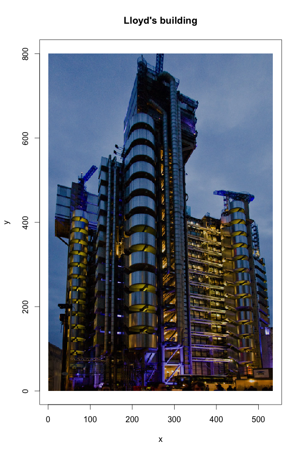

Running a k-means analysis on the three colour columns in my data frame allows me to reduce the picture to k colours. The output gives me for each x and y coordinate the colour cluster it belongs to. Thus, I plot my picture again, but replace the original colours with the cluster colours.