How to use optim in R
A friend of mine asked me the other day how she could use the function
The function
I start with a linear regression by minimising the residual sum of square and discuss how to carry out a maximum likelihood estimation in the second example.

optim in R to fit data. Of course there are built-in functions for fitting data in R and I wrote about this earlier. However, she wanted to understand how to do this from scratch using optim. The function
optim provides algorithms for general-purpose optimisations and the documentation is perfectly reasonable, but I remember that it took me a little while to get my head around how to pass data and parameters to optim. Thus, here are two simple examples.I start with a linear regression by minimising the residual sum of square and discuss how to carry out a maximum likelihood estimation in the second example.
Minimise residual sum of squares
I start with an x-y data set, which I believe has a linear relationship and therefore I'd like to fit y against x by minimising the residual sum of squares.dat=data.frame(x=c(1,2,3,4,5,6),
y=c(1,3,5,6,8,12))
y = par[1] + par[2] * x.min.RSS <- function(data, par) {
with(data, sum((par[1] + par[2] * x - y)^2))
}optim are the parameters I'd like to vary, par in this case; the second argument is the function to be minimised, min.RSS. The tricky bit is to understand how to apply optim to your data. The solution is the ... argument in optim, which allows me to pass other arguments through to min.RSS, here my data. Therefore I can use the following statement:result <- optim(par = c(0, 1), min.RSS, data = dat)
# I find the optimised parameters in result$par
# the minimised RSS is stored in result$value
result
## $par
## [1] -1.267 2.029
##
## $value
## [1] 2.819
##
## $counts
## function gradient
## 89 NA
##
## $convergence
## [1] 0
##
## $message
## NULLplot(y ~ x, data = dat, main="Least square regression")
abline(a = result$par[1], b = result$par[2], col = "red")Create an R package from a single R file with roxyPackage
Documenting code can be a bit of a pain. Yet, the older (and wiser?) I get, the more I realise how important it is. When I was younger I said 'documentation is for people without talent'. Well, I am clearly loosing my talent, as I sometimes struggle to understand what I programmed years ago. Thus, anything that soothes the pain of writing and maintaining documentation must be good and should help me to better understand my 'old me' in the future.
Ideally I want my R code and documentation in as few files as possible. A good start to achieve this is using roxygen2, an R package which has been around for some time. It allows me to tie R code together with the documentation in the same file and helps considerably in maintaining R packages.
The roxyPackage by Meik Michalke goes a step further, building on roxygen2. Meik presented his package at the Cologne R user group meeting a few weeks ago and I was intrigued by it. As I said in my notes to the meeting, with roxyPackage I can create a package from a single file of R code and documentation.
Here is an example of one R file to build a package using roxyPackage. For my toy example I wrote a doughnut plot function in R, something which is clearly missing ;)

I took the basic pie chart function and amended it to plot another white disc in the middle. On top of the function code I wrote the help file documentation using the roxygen2 syntax.
Ideally I want my R code and documentation in as few files as possible. A good start to achieve this is using roxygen2, an R package which has been around for some time. It allows me to tie R code together with the documentation in the same file and helps considerably in maintaining R packages.
The roxyPackage by Meik Michalke goes a step further, building on roxygen2. Meik presented his package at the Cologne R user group meeting a few weeks ago and I was intrigued by it. As I said in my notes to the meeting, with roxyPackage I can create a package from a single file of R code and documentation.
Here is an example of one R file to build a package using roxyPackage. For my toy example I wrote a doughnut plot function in R, something which is clearly missing ;)

I took the basic pie chart function and amended it to plot another white disc in the middle. On top of the function code I wrote the help file documentation using the roxygen2 syntax.
doughnut
,
End User Computing
,
R
,
roxygen2
,
roxyPackage
First steps of using googleVis on shiny
The guys at RStudio have done a fantastic job with shiny. It is really easy to build web apps with R using shiny. With the help of Joe Cheng from RStudio we figured out a way to make googleVis work on shiny as well. This allows you to make use of the Google Charts Tools in your shiny app directly from R. What I present here are three initial examples which seem to work in most browsers. The third example even uses a neat trick to create an animated geo chart.

However, before we upload the next version of googleVis to CRAN we decided to present a preview of version 0.4.0 here, asking for feedback. It would not be fair on the guys behind CRAN to release something into the wild, only to be told by users within a few days that we missed something. Hence, you can get the new version of googleVis only from the download page of our project site for the time being.
You may have read the post on RStudio's blog that the shiny API changed slightly: the
To run the following examples you need shiny version 0.4.0 and googleVis version 0.4.0 or higher.

However, before we upload the next version of googleVis to CRAN we decided to present a preview of version 0.4.0 here, asking for feedback. It would not be fair on the guys behind CRAN to release something into the wild, only to be told by users within a few days that we missed something. Hence, you can get the new version of googleVis only from the download page of our project site for the time being.
You may have read the post on RStudio's blog that the shiny API changed slightly: the
reactivePlot and reactiveText functions have been renamed to renderPlot and renderText with simplified input parameters. Thanks to Joe, there is now also a renderGvis function as part of the googleVis package, which works in very much the same way as the other two. To run the following examples you need shiny version 0.4.0 and googleVis version 0.4.0 or higher.
animation
,
googleVis
,
gvisGeoChart
,
gvisScatterChart
,
gvisTable
,
map
,
R
,
RStudio
,
shiny
,
Tutorials
Registration for 'R in Insurance' conference has opened

The registration for the first conference on R in Insurance on Monday 15 July 2013 at Cass Business School in London has opened.
The intended audience of the conference includes both academics and practitioners who are active or interested in the applications of R in insurance.
The 2013 R in Insurance conference builds upon the success of the R in Finance and R/Rmetrics events. We expect invited keynote lectures by:
- Professor Alexander McNeil, Department of Actuarial Science & Statistics
Heriot-Watt University: Implementing CreditRisk+ in R with the Faster Fourier Transform - Trevor Maynard, Head of Exposure Management and Reinsurance, Lloyd's: There is an R in Lloyd's
The submission deadline for abstracts is 28 March 2013. Please email your abstract (in txt or pdf format) to rinsuranceconference at gmail dot com.
The conference committee consists of:
Details about the registration and abstract submission are given on the new dedicated R in Insurance page at Cass Business School.
The organisers, Andreas Tsanakas and Markus Gesmann, gratefully acknowledge the sponsorship of Mango Solutions.
2013
,
Cass Business School
,
Conference
,
Insurance
,
News
,
R
,
R in Insurance
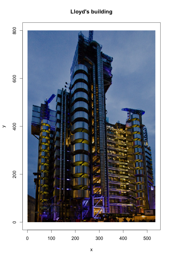
New Data Scientist role at Lloyd's
Lloyd's of London is looking for a Data Scientist as part of the Analysis team. See Lloyd's career web site for more details.

Review: Kölner R Meeting 6 February 2013
The fourth Cologne R user meeting took place last Wednesday at the Institute of Sociology. Thanks to Bernd Weiß for hosting the event and Revolution Analytics for their sponsorship.
We had two fantastic talks by Klaus Jacobi and M.eik Michalke. Klaus talked about Eliminating cloud pixels in satellite images via chronological interpolation and Meik presented his new roxyPackage package, which makes it even easier to maintain R packages with roxygen2.
About half of the fresh water in some regions of Pakistan is sourced from snow meting during the spring season. The water is captured in dams and as the snow only melts slowly the water supply is much more predictable than the water from the monsoon season, which is the other key source of fresh water during the year.
We had two fantastic talks by Klaus Jacobi and M.eik Michalke. Klaus talked about Eliminating cloud pixels in satellite images via chronological interpolation and Meik presented his new roxyPackage package, which makes it even easier to maintain R packages with roxygen2.
Eliminating cloud pixels in satellite images via chronological interpolation
Klaus gave a great case study about his consulting work as a water engineer in Asia, where he used R to analyse the snow melting process in the mountains of Pakistan. |
| Images of snow melting over time. Klaus Jacobi |
About half of the fresh water in some regions of Pakistan is sourced from snow meting during the spring season. The water is captured in dams and as the snow only melts slowly the water supply is much more predictable than the water from the monsoon season, which is the other key source of fresh water during the year.
Next Kölner R User Meeting: 6 February 2013
Quick reminder: The next Cologne R user group meeting is scheduled for tomorrow, 6 February 2013. All details and the agenda are available on the KölnRUG Meetup site. Please sign up if you would like to come along. Notes from the last Cologne R user group meeting are available here.

Thanks also to Revolution Analytics, who are sponsoring the Cologne R user group as part of their vector programme.
Kölner R Users
,
KölnR
,
News
,
R
,
Soapbox


