Showing posts with label Bayesian. Show all posts
Showing posts with label Bayesian. Show all posts
Notes from 4th Bayesian Mixer Meetup
Last Tuesday we got together for the 4th Bayesian Mixer Meetup. Product Madness kindly hosted us at their offices in Euston Square. About 50 Bayesians came along; the biggest turn up thus far, including developers of PyMC3 (Peadar Coyle) and Stan (Michael Betancourt).
The agenda had two feature talks by Dominic Steinitz and Volodymyr Kazantsev and a lightning talk by Jon Sedar.
Dominic shared with us his experience of using Hamiltonian and Sequential Monte Carlo samplers to model ecosystems.
Finding the 'best' model was Volodymyr's challenge. He tried various R packages (BMA, BMS and BAS) for Bayesian model averaging, with various degrees of success.
Finally, Jon gave a brief overview on Daft, a nifty Python package for creating graphs, or plate notation.
The agenda had two feature talks by Dominic Steinitz and Volodymyr Kazantsev and a lightning talk by Jon Sedar.
 |
| Dominic Steinitz: Hamiltonian and Sequential MC samplers to model ecosystems |
 |
| Volodymyr Kazantsev: Bayesian Model Averaging |
 |
| Jon Sedar: Easier Plate Notation in Python using Daft |
Next meeting
The next Bayesian Mixer Meetup meeting is already scheduled for 21 October. We will be back at Cass Business School, with two talks:- Darren Wilkinson: Hierarchical Bayesian Modelling of Growth Curves inc Stochastic Processes
- Peadar Coyle: Advanced PyMC3
Bayesian
,
Bayesian Mixer
,
Daft
,
Dynamical Systems
,
Model Averaging
,
python
,
R
,
Stan
Fitting a distribution in Stan from scratch
Last week the French National Institute of Health and Medical Research (Inserm) organised with the Stan Group a training programme on Bayesian Inference with Stan for Pharmacometrics in Paris.
Daniel Lee and Michael Betancourt, who run the course over three days, are not only members of Stan's development team, but also excellent teachers. Both were supported by Eric Novik, who gave an Introduction to Stan at the Paris Dataiku User Group last week as well.
I have been playing around with Stan on and off for some time, but as Eric pointed out to me, Stan is not that kind of girl(boy?). Indeed, having spent three days working with Stan has revitalised my relationship. Getting down to the basics has been really helpful and I shall remember, Stan is not drawing samples from a distribution. Instead, it is calculating the joint distribution function (in log space), and evaluating the probability distribution function (in log space).
Thus, here is a little example of fitting a set of random numbers in R to a Normal distribution with Stan. Yet, instead of using the built-in functions for the Normal distribution, I define the log probability function by hand, which I will use in the model block as well, and even generate a random sample, starting with a uniform distribution. However, I do use pre-defined distributions for the priors.
Why do I want to do this? This will be a template for the day when I have to use a distribution, which is not predefined in Stan, e.g. the actuar package has some interesting candidates.
I then use the Stan script to fit the data, i.e. to find the the parameters \(\mu\) and \(\sigma\), assuming that the data was generated by a Gaussian process.
The posterior parameter distributions include both \(\mu\) and \(\sigma\) in the 95% credible interval. The distribution of posterior predictive check (
Daniel Lee and Michael Betancourt, who run the course over three days, are not only members of Stan's development team, but also excellent teachers. Both were supported by Eric Novik, who gave an Introduction to Stan at the Paris Dataiku User Group last week as well.
 |
| Eric Kramer (Dataiku), Daniel Lee, Eric Novik & Michael Betancourt (Stan Group) |
I have been playing around with Stan on and off for some time, but as Eric pointed out to me, Stan is not that kind of girl(boy?). Indeed, having spent three days working with Stan has revitalised my relationship. Getting down to the basics has been really helpful and I shall remember, Stan is not drawing samples from a distribution. Instead, it is calculating the joint distribution function (in log space), and evaluating the probability distribution function (in log space).
Thus, here is a little example of fitting a set of random numbers in R to a Normal distribution with Stan. Yet, instead of using the built-in functions for the Normal distribution, I define the log probability function by hand, which I will use in the model block as well, and even generate a random sample, starting with a uniform distribution. However, I do use pre-defined distributions for the priors.
Why do I want to do this? This will be a template for the day when I have to use a distribution, which is not predefined in Stan, e.g. the actuar package has some interesting candidates.
Testing
I start off by generating fake data, a sample of 100 random numbers drawn from a Normal distribution with a mean of 4 and a standard deviation of 2. Note, the sample mean of the 100 figures is 4.2 and not 4. |
| Histogram of 100 random numbers drawn from N(4,2). |
 |
| Traceplot of 4 chains, including warm-up phase |
 |
| Histograms of posterior parameter and predictive samples |
 |
| Comparison of the emperical distributions |
y_ppc) is wider, taking into account the uncertainty of the parameters. The interquartile range and mean of my initial fake data and the sample of the posterior predictive distribution look very similar. That's good, my model generates data, which looks like the original data.Bayesian Mixer Meetup
Btw, tonight we have the 4th Bayesian Mixer Meetup in London.Session Info
R version 3.3.1 (2016-06-21)
Platform: x86_64-apple-darwin13.4.0 (64-bit)
Running under: OS X 10.12 (Sierra)

locale:
[1] en_GB.UTF-8/en_GB.UTF-8/en_GB.UTF-8/C/en_GB.UTF-8/en_GB.UTF-8

attached base packages:
[1] stats graphics grDevices utils datasets methods base

other attached packages:
[1] MASS_7.3-45 rstan_2.12.1 StanHeaders_2.12.0 ggplot2_2.1.0

loaded via a namespace (and not attached):
 [1] Rcpp_0.12.7      codetools_0.2-14 digest_0.6.10    grid_3.3.1
 [5] plyr_1.8.4       gtable_0.2.0     stats4_3.3.1     scales_0.4.0
 [9] labeling_0.3     tools_3.3.1      munsell_0.4.3    inline_0.3.14
[13] colorspace_1.2-6 gridExtra_2.2.1
Actuarial
,
Bayesian
,
fit distribution
,
R
,
Stan
Notes from 3rd and 3.5th Bayesian Mixer Meetup
Two Bayesian Mixer meet-ups in a row. Can it get any better?
Our third 'regular' meeting took place at Cass Business School on 24 June. Big thanks to Pietro and Andreas, who supported us from Cass. The next day, Jon Sedar of Applied AI, managed to arrange a special summer PyMC3 event.
We were lucky to have Robert Cowell talking to us, in what was his final week at Cass. Robert has been very much at the forefront of Bayesian development over the last 30 years. He is one of the co-authors of Probabilistic Networks and Expert Systems. Robert gave an insightful talk on probabilistic models for analysing mixed DNA traces. For illustration purpose, he used a crime case, where a man was killed in a pub, and where blood traces were used to support identifying the murder - turning statistics into a thriller.
Following those two stimulating talks, we had a few networking drinks at the Artillery Arms. But not too many, as the next day continued with another Bayesian event.
We had two core contributors with us: Chris Fonnesbeck (usually in Nashville, USA) and Thomas Wiecki (online from Düsseldorf, Germany), plus other package contributors.
On Saturday morning Chris gave an overview of PyMC3, followed by a detailed talk of Thomas on Bayesian Deep Learning. The afternoon was spent hacking together away on different problems. I was new to PyMC3, so I went through the tutorial on Probabilistic Programming using PyMC3, which Chris had given at a workshop in Oslo.
Many thanks to all who helped to make these events such a success and especially to Chris, Thomas, Luis, Robert, Andreas, Pietro and Jon.
If you have ideas for a future event, then please get in touch and visit our Meetup page.
Our third 'regular' meeting took place at Cass Business School on 24 June. Big thanks to Pietro and Andreas, who supported us from Cass. The next day, Jon Sedar of Applied AI, managed to arrange a special summer PyMC3 event.
3rd Bayesian Mixer meet-up
First up was Luis Usier, who talked about cross validation. Luis is a former student of Andrew Gelman, so, of course, his talk touched on Stan and the 'loo' (leave one out) package in R. Luis started with a simple artificial example that aimed to predict the probability of goalkeepers to save a shot on target. Adding a hierarchical structure to the model and treating the variance as a random variable, resulted in a pathological posterior distribution, which makes sampling next to impossible. Instead, fitting different models, with different fixed parameters, allows the user then to compare the models via cross-validation using the 'loo' function. Clever! I need to learn more about this. Luis' slides are available here and the underlying source code on GitHub. |
| Luis Usier talking about cross-validation in R and Stan |
We were lucky to have Robert Cowell talking to us, in what was his final week at Cass. Robert has been very much at the forefront of Bayesian development over the last 30 years. He is one of the co-authors of Probabilistic Networks and Expert Systems. Robert gave an insightful talk on probabilistic models for analysing mixed DNA traces. For illustration purpose, he used a crime case, where a man was killed in a pub, and where blood traces were used to support identifying the murder - turning statistics into a thriller.
Following those two stimulating talks, we had a few networking drinks at the Artillery Arms. But not too many, as the next day continued with another Bayesian event.
3.5th Meetup: PyMC3 summer special
We had a rare opportunity to gather together a few of the core contributors of the PyMC3 package for a talks & hack session. PyMC3 is a leading framework for probabilistic programming entirely based in Python with a 'theano' backend, with support for the NUTS sampler, Variational Inference and lots of useful functionality - an alternative to Stan.We had two core contributors with us: Chris Fonnesbeck (usually in Nashville, USA) and Thomas Wiecki (online from Düsseldorf, Germany), plus other package contributors.
 |
| Chris Fonnesbeck talking about PyMC3 |
On Saturday morning Chris gave an overview of PyMC3, followed by a detailed talk of Thomas on Bayesian Deep Learning. The afternoon was spent hacking together away on different problems. I was new to PyMC3, so I went through the tutorial on Probabilistic Programming using PyMC3, which Chris had given at a workshop in Oslo.
Many thanks to all who helped to make these events such a success and especially to Chris, Thomas, Luis, Robert, Andreas, Pietro and Jon.
If you have ideas for a future event, then please get in touch and visit our Meetup page.
Notes from 2nd Bayesian Mixer Meetup
Last Friday the 2nd Bayesian Mixer Meetup (@BayesianMixer) took place at Cass Business School, thanks to Pietro Millossovich and Andreas Tsanakas, who helped to organise the event.
 |
| Bayesian Mixer at Cass |
First up was Davide De March talking about the challenges in biochemistry experimentation, which are often characterised by complex and emerging relations among components.
The very little prior knowledge about complex molecules bindings left a fertile field for a probabilistic graphical model. In particular, Bayesian networks can help the investigator in the definition of a conditional dependence/independence structure where a joint multivariate probability distribution is determined. Hence, the use of Bayesian network can lead to a more efficient way of designing experiments.
 |
Davide De March: Bayesian Networks to design optimal experiments |
The second act of the night was Mick Cooney, presenting ideas of using growth curves to estimate the ultimate amounts paid in insurance by some cohort of policies.
The talk showed a model for these curves, discussed the implementation in Stan and how posterior predictive checks can be used to assess the output of the model.
 |
| Mick Cooney: Bayesian Modelling for Loss Curves in Insurance |
Thanks again to everyone who helped to make the event a success, particularly our speakers and Jon Sedar of Applied AI.
We are planning to run another event in mid-June. Please get in touch via our Meetup site with ideas and talk proposals.
Bayesian Mixer on Meetup
We had our first successful Bayesian Mixer Meetup last Friday night at the Artillery Arms!
We expected about 15 - 20 people to turn up, when we booked the function room overlooking Bunhill Cemetery and Bayes' grave. Now, looking at the photos taken during the evening, it seems that our prior believe was pretty good.

The event started with a talk from my side about some very basic Bayesian models, which I used a while back to get my head around the concepts in an insurance context. My talk "Experience vs Data" was based on presentations I had given last year at LondonR and the Warsaw R user group.
Jon Sedar followed with a fascinating talk about outlier detection using PyMC3.
Suppose, you have a bunch of data points, most of them centred, but with some further away. How do you decide if they are outliers, or not?
This question sounds very relevant to me in the insurance context as well. I have heard stories of underwriters telling me that certain years or events (meaning costly losses) were freaks, and should be disregarded, or in other words, without those losses the underwriter would have made a huge profit. I am not sure, I buy those arguments, as they undermine the fundamental business proposition of insurance; to pay, when policyholders experience 'freak' events. I am getting on my soap box, which I shouldn't.
We had a good night, very good discussions and some drinks. As a result Jon and I are committed to organise another event.
Jon has already set up a Meetup page, so please register online and get in touch with ideas, venues, talks, etc.
We expected about 15 - 20 people to turn up, when we booked the function room overlooking Bunhill Cemetery and Bayes' grave. Now, looking at the photos taken during the evening, it seems that our prior believe was pretty good.

The event started with a talk from my side about some very basic Bayesian models, which I used a while back to get my head around the concepts in an insurance context. My talk "Experience vs Data" was based on presentations I had given last year at LondonR and the Warsaw R user group.
Jon Sedar followed with a fascinating talk about outlier detection using PyMC3.
Suppose, you have a bunch of data points, most of them centred, but with some further away. How do you decide if they are outliers, or not?
This question sounds very relevant to me in the insurance context as well. I have heard stories of underwriters telling me that certain years or events (meaning costly losses) were freaks, and should be disregarded, or in other words, without those losses the underwriter would have made a huge profit. I am not sure, I buy those arguments, as they undermine the fundamental business proposition of insurance; to pay, when policyholders experience 'freak' events. I am getting on my soap box, which I shouldn't.
We had a good night, very good discussions and some drinks. As a result Jon and I are committed to organise another event.
Jon has already set up a Meetup page, so please register online and get in touch with ideas, venues, talks, etc.
Slides/Files
First Bayesian Mixer Meeting in London
There is a nice pub between Bunhill Fields and the Royal Statistical Society in London: The Artillery Arms. Clearly, the perfect place to bring people together to talk about Bayesian Statistics. Well, that’s what Jon Sedar (@jonsedar, applied.ai) and I thought.
Hence, we’d like to organise a Bayesian Mixer Meetup on Friday, 12 February, 19:00. We booked the upstairs function room at the Artillery Arms and if you look outside the window, you can see Thomas Bayes’ grave.
We intend the group to be small (announcing only on the stan user group, pymc-devs gitter, and here for now) and geared to open discussion of Bayesian inference, tools, techniques and theory. Neither of us is a great expert, we're really just users of the tools, but we'd love to welcome academic discussion as well as real world examples etc.
Jon is more the Python/PyMC guy, while I come from the R/Rstan corner. We will prepare two talks to kick this off. Jon will talk about GLM Robust Regression with Outlier Detection using PyMC3, while I will talk about Experience vs Data with some stories from insurance and actuarial science, sprinkled with RStan examples.
If you would like to join us, please get in touch via the form below, so that we can keep tabs on numbers, and if this goes all well we shall set up a Meetup site.
 |
| Source: http://www.artillery-arms.co.uk/ |
We intend the group to be small (announcing only on the stan user group, pymc-devs gitter, and here for now) and geared to open discussion of Bayesian inference, tools, techniques and theory. Neither of us is a great expert, we're really just users of the tools, but we'd love to welcome academic discussion as well as real world examples etc.
Jon is more the Python/PyMC guy, while I come from the R/Rstan corner. We will prepare two talks to kick this off. Jon will talk about GLM Robust Regression with Outlier Detection using PyMC3, while I will talk about Experience vs Data with some stories from insurance and actuarial science, sprinkled with RStan examples.
If you would like to join us, please get in touch via the form below, so that we can keep tabs on numbers, and if this goes all well we shall set up a Meetup site.
Loss Developments via Growth Curves and Stan
Last week I posted a biological example of fitting a non-linear growth curve with Stan/RStan. Today, I want to apply a similar approach to insurance data using ideas by David Clark [1] and James Guszcza [2].
Instead of predicting the growth of dugongs (sea cows), I would like to predict the growth of cumulative insurance loss payments over time, originated from different origin years. Loss payments of younger accident years are just like a new generation of dugongs, they will be small in size initially, grow as they get older, until the losses are fully settled.
Here is my example data set:
 Following the articles cited above I will assume that the growth can be explained by a Weibull curve, with two parameters \(\theta\) (scale) and \(\omega\) (shape):
\[
G(dev|\omega, \theta) = 1 - \exp\left(-\left(\frac{dev}{\theta}\right)^\omega\right)
\]Inspired by the classical over-dispersed Poisson GLM in actuarial science, Guszcza [2] assumes a power variance structure for the process error as well. For the purpose of this post I will assume that claims cost follow a Normal distribution, to make a comparison with a the classical least square regression easier. With a prior estimate of the ultimate claims cost the cumulative loss can be modelled as:
\[
\begin{align}
CL_{AY, dev} & \sim \mathcal{N}(\mu_{dev}, \sigma^2_{dev}) \\
\mu_{dev} & = Ult \cdot G(dev|\omega, \theta)\\
\sigma_{dev} & = \sigma \sqrt{\mu_{dev}}
\end{align}
\]Perhaps, the above formula suggests a hierarchical modelling approach, with different ultimate loss costs by accident year. Indeed, this is the focus of [2] and I will endeavour to reproduce the results with Stan in my next post, but today I will stick to a pooled model that assumes a constant ultimate loss across all accident years, i.e. \(Ult_{AY} = Ult \;\forall\; AY\).
To prepare my analysis I read in the data as a long data frame instead of the matrix structure above. Additionally, I compose another data frame that I will use later to predict payments two years beyond the first 10 years. Furthermore, to align the output with [2] I relabelled the development periods from years to months, so that year 1 becomes month 6, year 2 becomes month 18, etc. The accident years run from 1991 to 2000, while the variable
To get a reference point for Stan I start with a non-linear least square regression:
 The output above doesn't look unreasonable, apart from the accident years 1991, 1992 and 1998. The output of
The Stan code below is very similar to last week. Again, I am interested here in the posterior distributions, hence I add a block to generate quantities from those. Note, Stan comes with a build-in function for the cumulative Weibull distribution
I store the Stan code in a separate text file, which I read into R to compile the model. The compilation takes a little time. The sampling itself is done in a few seconds.
Let's take a look at the output:

 The parameters are a little different to the output of
Finally, I can plot the 90% credible intervals of the posterior distributions.
 The 90% prediction credible interval captures most of the data and although this model might not be suitable for reserving individual accident years, it could provide an initial starting point for further investigations. Additionally, thanks to the Bayesian model I have access to the full distribution, not just point estimators and standard errors.
My next post will continue with this data set and the ideas of James Guszcza by allowing the ultimate loss cost to vary by accident year, treating it as a random effect. Here is a teaser of what the output will look like:

[2] Guszcza, J. Hierarchical Growth Curve Models for Loss Reserving, 2008, CAS Fall Forum,
pp. 146–173.
Instead of predicting the growth of dugongs (sea cows), I would like to predict the growth of cumulative insurance loss payments over time, originated from different origin years. Loss payments of younger accident years are just like a new generation of dugongs, they will be small in size initially, grow as they get older, until the losses are fully settled.
Here is my example data set:
\[
G(dev|\omega, \theta) = 1 - \exp\left(-\left(\frac{dev}{\theta}\right)^\omega\right)
\]Inspired by the classical over-dispersed Poisson GLM in actuarial science, Guszcza [2] assumes a power variance structure for the process error as well. For the purpose of this post I will assume that claims cost follow a Normal distribution, to make a comparison with a the classical least square regression easier. With a prior estimate of the ultimate claims cost the cumulative loss can be modelled as:
\[
\begin{align}
CL_{AY, dev} & \sim \mathcal{N}(\mu_{dev}, \sigma^2_{dev}) \\
\mu_{dev} & = Ult \cdot G(dev|\omega, \theta)\\
\sigma_{dev} & = \sigma \sqrt{\mu_{dev}}
\end{align}
\]Perhaps, the above formula suggests a hierarchical modelling approach, with different ultimate loss costs by accident year. Indeed, this is the focus of [2] and I will endeavour to reproduce the results with Stan in my next post, but today I will stick to a pooled model that assumes a constant ultimate loss across all accident years, i.e. \(Ult_{AY} = Ult \;\forall\; AY\).
To prepare my analysis I read in the data as a long data frame instead of the matrix structure above. Additionally, I compose another data frame that I will use later to predict payments two years beyond the first 10 years. Furthermore, to align the output with [2] I relabelled the development periods from years to months, so that year 1 becomes month 6, year 2 becomes month 18, etc. The accident years run from 1991 to 2000, while the variable
origin maps those years from 1 to 10.To get a reference point for Stan I start with a non-linear least square regression:
gnls gives me an opportunity to provide my prior distributions with good starting points. I will use an inverse Gamma as a prior for \(\sigma\), constrained Normals for the parameters \(\theta, \omega\) and \(Ult\) as well. If you have better ideas, then please get in touch.The Stan code below is very similar to last week. Again, I am interested here in the posterior distributions, hence I add a block to generate quantities from those. Note, Stan comes with a build-in function for the cumulative Weibull distribution
weibull_cdf.I store the Stan code in a separate text file, which I read into R to compile the model. The compilation takes a little time. The sampling itself is done in a few seconds.
Let's take a look at the output:
gnls, but well within the standard error. From the plots I notice that the samples for the ultimate loss as well as for \(\theta\) are a little skewed to the right. Well, assuming cumulative losses to follow a Normal distribution was a bit a of stretch to start with. Still, the samples seem to converge.Finally, I can plot the 90% credible intervals of the posterior distributions.
My next post will continue with this data set and the ideas of James Guszcza by allowing the ultimate loss cost to vary by accident year, treating it as a random effect. Here is a teaser of what the output will look like:
References
[1] David R. Clark. LDF Curve-Fitting and Stochastic Reserving: A Maximum Likelihood Approach. Casualty Actuarial Society, 2003. CAS Fall Forum.[2] Guszcza, J. Hierarchical Growth Curve Models for Loss Reserving, 2008, CAS Fall Forum,
pp. 146–173.
Session Info
R version 3.2.2 (2015-08-14)
Platform: x86_64-apple-darwin13.4.0 (64-bit)
Running under: OS X 10.11.1 (El Capitan)

locale:
[1] en_GB.UTF-8/en_GB.UTF-8/en_GB.UTF-8/C/en_GB.UTF-8/en_GB.UTF-8

attached base packages:
[1] stats     graphics  grDevices utils     datasets  methods
[7] base

other attached packages:
[1] rstan_2.8.0    ggplot2_1.0.1     Rcpp_0.12.1
[4] nlme_3.1-122   lattice_0.20-33   ChainLadder_0.2.3

loaded via a namespace (and not attached):
 [1] nloptr_1.0.4       plyr_1.8.3         tools_3.2.2
 [4] digest_0.6.8       lme4_1.1-10        statmod_1.4.21
 [7] gtable_0.1.2       mgcv_1.8-8         Matrix_1.2-2
[10] parallel_3.2.2     biglm_0.9-1        SparseM_1.7
[13] proto_0.3-10       gridExtra_2.0.0    coda_0.18-1
[16] stringr_1.0.0      MatrixModels_0.4-1 stats4_3.2.2
[19] lmtest_0.9-34      grid_3.2.2         nnet_7.3-11
[22] inline_0.3.14      tweedie_2.2.1      cplm_0.7-4
[25] minqa_1.2.4        reshape2_1.4.1     car_2.1-0
[28] actuar_1.1-10      magrittr_1.5       codetools_0.2-14
[31] scales_0.3.0       MASS_7.3-44        splines_3.2.2
[34] systemfit_1.1-18   rsconnect_0.3.79   pbkrtest_0.4-2
[37] colorspace_1.2-6   labeling_0.3       quantreg_5.19
[40] sandwich_2.3-4     stringi_1.0-1      munsell_0.4.2
[43] zoo_1.7-12Bayesian regression models using Stan in R
It seems the summer is coming to end in London, so I shall take a final look at my ice cream data that I have been playing around with to predict sales statistics based on temperature for the last couple of weeks [1], [2], [3].
Here I will use the new
Thanks to
Let's start. Here is the data again:
My models are written down in very much the same way as with
Last week I wrote the Stan model for the log-transformed linear model myself. Here is the output of
I access the underlying Stan model via
To review the model I start by plotting the trace and density plots for the MCMC samples.

Combining the outputs of all four models into one data frame gives me then the opportunity to compare the prediction credible intervals of the four models in one chart.

There are no big news in respect of the four models, but for the fact that here I can look at the posterior prediction credible intervals, rather then the theoretical distributions two weeks ago. The over-prediction of the log-transformed linear model is apparent again.
Well, if I set the probability of selling out at 2.5%, then I will have enough ice cream to sell with 97.5% certainty. To estimate those statistics I have to calculate the 97.5% percentile of the posterior predictive samples.
 Ok, I have four models and four answers ranging from 761 to 2494. The highest number is more than 3 times the lowest number!
I had set the market size at 800 in my binomial model, so I am not surprised by its answer of 761. Also, I noted earlier that the log-normal distribution is skewed to the right, so that explains the high prediction of 2494. The Poisson model, like the log-transform linear model, has the implicit exponential growth assumption. Its mean forecast is well over 1000 as I pointed out earlier and hence the 97.5% prediction of 1510 is to be expected.
Another aspect to consider would be the cost of holding unsold stock. Ice cream can usually be stored for some time, but the situation would be quite different for freshly baked bread or bunches of flowers that have to be sold quickly.
Here I will use the new
brms (GitHub, CRAN) package by Paul-Christian Bürkner to derive the 95% prediction credible interval for the four models I introduced in my first post about generalised linear models. Additionally, I am interested to predict how much ice cream I should hold in stock for a hot day at 35ºC, such that I only run out of ice cream with a probability of 2.5%.Stan models with brms
Like in my previous post about the log-transformed linear model with Stan, I will use Bayesian regression models to estimate the 95% prediction credible interval from the posterior predictive distribution.Thanks to
brms this will take less than a minute of coding, because brm allows me to specify my models in the usual formula syntax and I can leave it to the package functions to create and execute the Stan files.Let's start. Here is the data again:
My models are written down in very much the same way as with
glm. Only the binomial model requires a slightly different syntax. Here I use the default priors and link functions:Last week I wrote the Stan model for the log-transformed linear model myself. Here is the output of
brm. The estimated parameters are quite similar, apart from \(\sigma\):I access the underlying Stan model via
log.lin.mod$model and note that the prior of \(\sigma\) is modelled via a Cauchy distribution, unlike the inverse Gamma I used last week. I believe that explains my small difference in \(\sigma\).To review the model I start by plotting the trace and density plots for the MCMC samples.
Prediction credible interval
Thepredict function gives me access to the posterior predictive statistics, including the 95% prediction credible interval. Combining the outputs of all four models into one data frame gives me then the opportunity to compare the prediction credible intervals of the four models in one chart.
There are no big news in respect of the four models, but for the fact that here I can look at the posterior prediction credible intervals, rather then the theoretical distributions two weeks ago. The over-prediction of the log-transformed linear model is apparent again.
How much stock should I hold on a hot day?
Running out of stock on a hot summer's day would be unfortunate, because those are days when sells will be highest. But how much stock should I hold?Well, if I set the probability of selling out at 2.5%, then I will have enough ice cream to sell with 97.5% certainty. To estimate those statistics I have to calculate the 97.5% percentile of the posterior predictive samples.
I had set the market size at 800 in my binomial model, so I am not surprised by its answer of 761. Also, I noted earlier that the log-normal distribution is skewed to the right, so that explains the high prediction of 2494. The Poisson model, like the log-transform linear model, has the implicit exponential growth assumption. Its mean forecast is well over 1000 as I pointed out earlier and hence the 97.5% prediction of 1510 is to be expected.
Conclusions
How much ice cream should I hold in stock? Well, if I believe strongly in my assumption of a market size of 800, then I should stick with the output of the binomial model, or perhaps hold 800 just in case.Another aspect to consider would be the cost of holding unsold stock. Ice cream can usually be stored for some time, but the situation would be quite different for freshly baked bread or bunches of flowers that have to be sold quickly.
Session Info
Note, I used the developer version ofbrms from GitHub.R version 3.2.2 (2015-08-14)
Platform: x86_64-apple-darwin13.4.0 (64-bit)
Running under: OS X 10.10.5 (Yosemite)
locale:
[1] en_GB.UTF-8/en_GB.UTF-8/en_GB.UTF-8/C/en_GB.UTF-8/en_GB.UTF-8
attached base packages:
[1] stats graphics grDevices utils datasets
[6] methods base
other attached packages:
[1] lattice_0.20-33 brms_0.4.1.9000 ggplot2_1.0.1
[4] rstan_2.7.0-1 inline_0.3.14 Rcpp_0.12.0
loaded via a namespace (and not attached):
[1] codetools_0.2-14 digest_0.6.8 MASS_7.3-43
[4] grid_3.2.2 plyr_1.8.3 gtable_0.1.2
[7] stats4_3.2.2 magrittr_1.5 scales_0.2.5
[10] stringi_0.5-5 reshape2_1.4.1 proto_0.3-10
[13] tools_3.2.2 stringr_1.0.0 munsell_0.4.2
[16] parallel_3.2.2 colorspace_1.2-6Posterior predictive output with Stan
I continue my Stan experiments with another insurance example. Here I am particular interested in the posterior predictive distribution from only three data points. Or, to put it differently I have a customer of three years and I'd like to predict the expected claims cost for the next year to set or adjust the premium.
The example is taken from section 16.17 in Loss Models: From Data to Decisions [1]. Some time ago I used the same example to get my head around a Bayesian credibility model.
Suppose the claims likelihood distribution is believed to follow an exponential distribution for a given parameter \(\Theta\). The prior parameter distribution on \(\Theta\) is assumed to be a gamma distribution with parameters \(\alpha=4, \beta=1000\):
\[\begin{aligned}\Theta & \sim \mbox{Gamma}(\alpha, \beta)\\
\ell_i & \sim \mbox{Exp}(\Theta) , \; \forall i \in N
\end{aligned}\]In this case the predictive distribution is a Pareto II distribution with density \(f(x) = \frac{\alpha \beta^\alpha}{(x+\beta)^{\alpha+1}}\) and a mean of \(\frac{\beta}{\alpha-1}=\,\)333.33.
I have three independent observations, namely losses of $100, $950 and $450. The posterior predictive expected loss is $416.67 and can be derived analytical, as shown in my earlier post. Now let me reproduce the answer with Stan as well.
Implementing the model in Stan is straightforward and I follow the same steps as in my simple example of last week. However, here I am also interested in the posterior predictive distribution, hence I add a

The output shows a simulated predictive mean of $416.86, close to the analytical answer. I can also read out that the 75%ile of the posterior predictive distribution is a loss of $542 vs. $414 from the prior predictive. That means every four years I shouldn't be surprised to observe a loss in excess of $500. Further I note that 90% of losses are expected to be less than $950, or in other words the observation in my data may reflect the outcome of an event with a 1 in 10 return period.
Comparing the sampling output from Stan with the analytical output gives me some confidence that I am doing the 'right thing'.
The example is taken from section 16.17 in Loss Models: From Data to Decisions [1]. Some time ago I used the same example to get my head around a Bayesian credibility model.
Suppose the claims likelihood distribution is believed to follow an exponential distribution for a given parameter \(\Theta\). The prior parameter distribution on \(\Theta\) is assumed to be a gamma distribution with parameters \(\alpha=4, \beta=1000\):
\[\begin{aligned}\Theta & \sim \mbox{Gamma}(\alpha, \beta)\\
\ell_i & \sim \mbox{Exp}(\Theta) , \; \forall i \in N
\end{aligned}\]In this case the predictive distribution is a Pareto II distribution with density \(f(x) = \frac{\alpha \beta^\alpha}{(x+\beta)^{\alpha+1}}\) and a mean of \(\frac{\beta}{\alpha-1}=\,\)333.33.
I have three independent observations, namely losses of $100, $950 and $450. The posterior predictive expected loss is $416.67 and can be derived analytical, as shown in my earlier post. Now let me reproduce the answer with Stan as well.
Implementing the model in Stan is straightforward and I follow the same steps as in my simple example of last week. However, here I am also interested in the posterior predictive distribution, hence I add a
generated quantities code block. The output shows a simulated predictive mean of $416.86, close to the analytical answer. I can also read out that the 75%ile of the posterior predictive distribution is a loss of $542 vs. $414 from the prior predictive. That means every four years I shouldn't be surprised to observe a loss in excess of $500. Further I note that 90% of losses are expected to be less than $950, or in other words the observation in my data may reflect the outcome of an event with a 1 in 10 return period.
Comparing the sampling output from Stan with the analytical output gives me some confidence that I am doing the 'right thing'.
References
[1] Klugman, S. A., Panjer, H. H. & Willmot, G. E. (2004), Loss Models: From Data to Decisions, Wiley Series in Probability and Statistics.Session Info
R version 3.2.0 (2015-04-16)
Platform: x86_64-apple-darwin13.4.0 (64-bit)
Running under: OS X 10.10.3 (Yosemite)

locale:
[1] en_GB.UTF-8/en_GB.UTF-8/en_GB.UTF-8/C/en_GB.UTF-8/en_GB.UTF-8

attached base packages:
[1] stats graphics grDevices utils datasets methods base

other attached packages:
[1] lattice_0.20-31 actuar_1.1-8 rstan_2.6.0 inline_0.3.14
[5] Rcpp_0.11.6

loaded via a namespace (and not attached):
[1] tools_3.2.0  codetools_0.2-11 grid_3.2.0 stats4_3.2.0
Hello Stan!
In my previous post I discussed how Longley-Cook, an actuary at an insurance company in the 1950's, used Bayesian reasoning to estimate the probability for a mid-air collision of two planes.
Here I will use the same model to get started with Stan/RStan, a probabilistic programming language for Bayesian inference.
Last week my prior was given as a Beta distribution with parameters \(\alpha=1, \beta=1\) and the likelihood was assumed to be a Bernoulli distribution with parameter \(\theta\):
\[\begin{aligned}
\theta & \sim \mbox{Beta}(1, 1)\\
y_i & \sim \mbox{Bernoulli}(\theta), \;\forall i \in N
\end{aligned}\]For the previous five years no mid-air collision were observed, \(x=\{0, 0, 0, 0, 0\}\). That's my data.
In this case the posterior distributions can be derived analytically. The posterior hyper-parameters are \(\alpha'=\alpha + \sum_{i=1}^n x_i,\, \beta'=\beta + n - \sum_{i=1}^n x_i\) and with that I get the posterior parameter for the predictive distribution, which is a Bernoulli distribution again: \(\theta' = \alpha'/(\alpha'+\beta')=1/7\approx14.3\%\).
Still, I can use Stan and MCMC simulations to come to the same answers (of course I am using a sledgehammer here to crack a nut).
In the first code block the model is written in Stan's modelling language. The next section calls

Interested in the application of R in insurance? Join us at the 3rd R in Insurance conference in Amsterdam, 29 June 2015.
Here I will use the same model to get started with Stan/RStan, a probabilistic programming language for Bayesian inference.
Last week my prior was given as a Beta distribution with parameters \(\alpha=1, \beta=1\) and the likelihood was assumed to be a Bernoulli distribution with parameter \(\theta\):
\[\begin{aligned}
\theta & \sim \mbox{Beta}(1, 1)\\
y_i & \sim \mbox{Bernoulli}(\theta), \;\forall i \in N
\end{aligned}\]For the previous five years no mid-air collision were observed, \(x=\{0, 0, 0, 0, 0\}\). That's my data.
In this case the posterior distributions can be derived analytically. The posterior hyper-parameters are \(\alpha'=\alpha + \sum_{i=1}^n x_i,\, \beta'=\beta + n - \sum_{i=1}^n x_i\) and with that I get the posterior parameter for the predictive distribution, which is a Bernoulli distribution again: \(\theta' = \alpha'/(\alpha'+\beta')=1/7\approx14.3\%\).
Still, I can use Stan and MCMC simulations to come to the same answers (of course I am using a sledgehammer here to crack a nut).
In the first code block the model is written in Stan's modelling language. The next section calls
stan and finally the results can be analysed. The answers are very much the same as the analytical approach in my previous post.Interested in the application of R in insurance? Join us at the 3rd R in Insurance conference in Amsterdam, 29 June 2015.
Session Info
R version 3.2.0 (2015-04-16)
Platform: x86_64-apple-darwin13.4.0 (64-bit)
Running under: OS X 10.10.3 (Yosemite)

locale:
[1] en_GB.UTF-8/en_GB.UTF-8/en_GB.UTF-8/C/en_GB.UTF-8/en_GB.UTF-8

attached base packages:
[1] stats     graphics  grDevices utils     datasets  methods   base

other attached packages:
[1] rstan_2.6.0   inline_0.3.14 Rcpp_0.11.6

loaded via a namespace (and not attached):
[1] tools_3.2.0 codetools_0.2-11 stats4_3.2.0Predicting events, when they haven't happened yet
Suppose you have to predict the probabilities of events which haven't happened yet. How do you do this?
Here is an example from the 1950s when Longley-Cook, an actuary at an insurance company, was asked to price the risk for a mid-air collision of two planes, an event which as far as he knew hadn't happened before. The civilian airline industry was still very young, but rapidly growing and all Longely-Cook knew was that there were no collisions in the previous 5 years [1].
Where do you start?
Although the probability for a mid-air collision should be very low for any given plane, the probability for an event in a year will be higher.
Let's think of the years as a series of Bernoulli trials with unknown probability \(p\). That's a likelihood. If I start with an uninformed prior, such as a Beta(\(\alpha,\beta\)) with \(\alpha=1, \beta=1\) then I can use the concept of Bayesian conjugates to update my prior believe.
In this case the posterior parameter distribution is Beta again with hyper-parameters \(\alpha'=\alpha + \sum_{i=1}^n x_i,\, \beta'=\beta + n - \sum_{i=1}^n x_i\), where \(x_i=1\) if the event occurred, or 0 otherwise and \(n\) is the number of years.
Thus, the updated parameters are \(\alpha'=1, \beta'=6\), with a posterior predictive mean of \(\alpha'/(\alpha'+\beta')=1/7\). That is a 14.3% chance for a mid-air collision in the next year with a 95% confidence interval of [0, 39%]. Or, in other words, if I round 39% to 40%, a return period of 2.5 years (1/0.4), i.e. up to 4 incidents in 10 years should be allowed for. That's what Longley-Cook predicted.
Tragically, 128 people died over the Grand Canyon in 1956, and 4 years after that, 134 people died over New York City.
Wikipedia lists 51 notable civilian mid-air collisions since 1922, including helicopters and space crafts. Since 1955 there were 11 incidents that had more than 100 fatalities, the last one in 2006.
So, what would this mean to Mr. Longley-Cook today? Well, first of all that his prediction wasn't too bad at all. Perhaps, he would set the probability at (1+11)/((1+11)+(1+60-11)\(\approx\)20% today. He may have argued that 2 x 20% = 40% of the average plane value should be included in the world wide premium for airline hull to cover mid-air collisions.

Interested in the application of R in insurance? Join us at the 3rd R in Insurance conference in Amsterdam, 29 June 2015.
Here is an example from the 1950s when Longley-Cook, an actuary at an insurance company, was asked to price the risk for a mid-air collision of two planes, an event which as far as he knew hadn't happened before. The civilian airline industry was still very young, but rapidly growing and all Longely-Cook knew was that there were no collisions in the previous 5 years [1].
Where do you start?
Although the probability for a mid-air collision should be very low for any given plane, the probability for an event in a year will be higher.
Let's think of the years as a series of Bernoulli trials with unknown probability \(p\). That's a likelihood. If I start with an uninformed prior, such as a Beta(\(\alpha,\beta\)) with \(\alpha=1, \beta=1\) then I can use the concept of Bayesian conjugates to update my prior believe.
In this case the posterior parameter distribution is Beta again with hyper-parameters \(\alpha'=\alpha + \sum_{i=1}^n x_i,\, \beta'=\beta + n - \sum_{i=1}^n x_i\), where \(x_i=1\) if the event occurred, or 0 otherwise and \(n\) is the number of years.
Thus, the updated parameters are \(\alpha'=1, \beta'=6\), with a posterior predictive mean of \(\alpha'/(\alpha'+\beta')=1/7\). That is a 14.3% chance for a mid-air collision in the next year with a 95% confidence interval of [0, 39%]. Or, in other words, if I round 39% to 40%, a return period of 2.5 years (1/0.4), i.e. up to 4 incidents in 10 years should be allowed for. That's what Longley-Cook predicted.
Tragically, 128 people died over the Grand Canyon in 1956, and 4 years after that, 134 people died over New York City.
Wikipedia lists 51 notable civilian mid-air collisions since 1922, including helicopters and space crafts. Since 1955 there were 11 incidents that had more than 100 fatalities, the last one in 2006.
So, what would this mean to Mr. Longley-Cook today? Well, first of all that his prediction wasn't too bad at all. Perhaps, he would set the probability at (1+11)/((1+11)+(1+60-11)\(\approx\)20% today. He may have argued that 2 x 20% = 40% of the average plane value should be included in the world wide premium for airline hull to cover mid-air collisions.
R code
Interested in the application of R in insurance? Join us at the 3rd R in Insurance conference in Amsterdam, 29 June 2015.
References
[1] Computational Actuarial Science with R, Edited by Arthur Charpentier, Chapman and Hall/CRC Reference - 656 PagesSession Info
R version 3.2.0 (2015-04-16)
Platform: x86_64-apple-darwin13.4.0 (64-bit)
Running under: OS X 10.10.3 (Yosemite)

locale:
[1] en_GB.UTF-8/en_GB.UTF-8/en_GB.UTF-8/C/en_GB.UTF-8/en_GB.UTF-8

attached base packages:
[1] stats     graphics  grDevices utils     datasets  methods
[7] base

other attached packages:
[1] XML_3.98-1.1

loaded via a namespace (and not attached):
[1] tools_3.2.0Extended Kalman filter example in R
Last week's post about the Kalman filter focused on the derivation of the algorithm. Today I will continue with the extended Kalman filter (EKF) that can deal also with nonlinearities. According to Wikipedia the EKF has been considered the de facto standard in the theory of nonlinear state estimation, navigation systems and GPS.
\[\begin{align}
x_{t+1} & = A x_t + w_t,\quad w_t \sim N(0,Q)\\
y_t &=G x_t + \nu_t, \quad \nu_t \sim N(0,R)\\
x_1 & \sim N(\hat{x}_0, \Sigma_0)
\end{align}
\]With \(x_t\) describing the state space evolution, \(y_t\) the observations, \(A, Q, G, R, \Sigma_0\) matrices of appropriate dimensions, \(w_t\) the evolution error and \(\nu_t\) the observation error. The Kalman filter provides recursive estimators for \(x_t\) via:
\[\begin{align}
K_{t} &= A \Sigma_t G' (G \Sigma_t G' + R)^{-1}\\
\hat{x}_{t+1} &= A \hat{x_t} + K_{t} (y_t - G \hat{x}_t) \\
\Sigma_{t+1} &= A \Sigma_t A' - K_{t} G \Sigma_t A' + Q
\end{align}\]In the case of nonlinearities on the right hand side of either the state (\(x_t\)) or observation (\(y_t\)) equation the extended Kalman filter uses a simple and elegant trick: Taylor series of the first order, or in other words, I simply linearise the right hand side. The matrices \(A\) and \(G\) will be the Jacobian matrices of the respected vector functions.
The logistic growth model can be written as a time-invariant dynamical system with growth rate \(r\) and carrying capacity \(k\):
\[
\begin{aligned}
\dot{p} & = r p\Big(1 - \frac{p}{k}\Big)
\end{aligned}
\]The above ordinary differential equation has the well known analytical solution:
\[
p = \frac{kp_0\exp(r\,t)}{k + p_0(\exp(r\,t) - 1)}
\]Suppose I observe data of a population for which I know the carrying capacity \(k\), but where the growth rate \(r\) is noisy.

\[
\begin{aligned}
r_i &= r_{i-1} \\
p_i &= \frac{kp_{i-1}\exp(r_{i-1}\Delta T)}{k + p_{i-1}(\exp(r_{i-1}\Delta T) - 1)} \\
y_i &= \begin{bmatrix}0 & 1\end{bmatrix} \begin{bmatrix}r_i \\
p_i\end{bmatrix} + \nu
\end{aligned}
\]Or with \(x_i:=\begin{bmatrix}r_i & p_i\end{bmatrix}'\) as:
\[
\begin{aligned}
x_i &= a(x_i)\\
y_i &= G x_i + \nu_i, \quad \nu_i \sim N(0,R)
\end{aligned}
\]In my example the state space model is purely deterministic, so there isn't any evolution noise and hence \(Q=0\).
With an initial prior guess for \(x_0\) and \(\Sigma_0\) and I am ready to go. The R code below shows my implementation with the algorithm above. Note that I use the
 After a few time steps the extended Kalman filter does a fantastic job in reducing the noise. Perhaps this shouldn't be too surprising as a local linearisation of the logistic growth function will give a good fit. The situation might be different for highly nonlinear functions. The Wikipedia article about the Kalman filter suggests the unscented version in those cases.
Kalman filter
I had the following dynamic linear model for the Kalman filter last week:\[\begin{align}
x_{t+1} & = A x_t + w_t,\quad w_t \sim N(0,Q)\\
y_t &=G x_t + \nu_t, \quad \nu_t \sim N(0,R)\\
x_1 & \sim N(\hat{x}_0, \Sigma_0)
\end{align}
\]With \(x_t\) describing the state space evolution, \(y_t\) the observations, \(A, Q, G, R, \Sigma_0\) matrices of appropriate dimensions, \(w_t\) the evolution error and \(\nu_t\) the observation error. The Kalman filter provides recursive estimators for \(x_t\) via:
\[\begin{align}
K_{t} &= A \Sigma_t G' (G \Sigma_t G' + R)^{-1}\\
\hat{x}_{t+1} &= A \hat{x_t} + K_{t} (y_t - G \hat{x}_t) \\
\Sigma_{t+1} &= A \Sigma_t A' - K_{t} G \Sigma_t A' + Q
\end{align}\]In the case of nonlinearities on the right hand side of either the state (\(x_t\)) or observation (\(y_t\)) equation the extended Kalman filter uses a simple and elegant trick: Taylor series of the first order, or in other words, I simply linearise the right hand side. The matrices \(A\) and \(G\) will be the Jacobian matrices of the respected vector functions.
Logistic growth
As an example I will use a logistic growth model, inspired by the Hakell example given by Dominic Steinitz.The logistic growth model can be written as a time-invariant dynamical system with growth rate \(r\) and carrying capacity \(k\):
\[
\begin{aligned}
\dot{p} & = r p\Big(1 - \frac{p}{k}\Big)
\end{aligned}
\]The above ordinary differential equation has the well known analytical solution:
\[
p = \frac{kp_0\exp(r\,t)}{k + p_0(\exp(r\,t) - 1)}
\]Suppose I observe data of a population for which I know the carrying capacity \(k\), but where the growth rate \(r\) is noisy.

Extended Kalman filter
The state space and observation model can then be written as:\[
\begin{aligned}
r_i &= r_{i-1} \\
p_i &= \frac{kp_{i-1}\exp(r_{i-1}\Delta T)}{k + p_{i-1}(\exp(r_{i-1}\Delta T) - 1)} \\
y_i &= \begin{bmatrix}0 & 1\end{bmatrix} \begin{bmatrix}r_i \\
p_i\end{bmatrix} + \nu
\end{aligned}
\]Or with \(x_i:=\begin{bmatrix}r_i & p_i\end{bmatrix}'\) as:
\[
\begin{aligned}
x_i &= a(x_i)\\
y_i &= G x_i + \nu_i, \quad \nu_i \sim N(0,R)
\end{aligned}
\]In my example the state space model is purely deterministic, so there isn't any evolution noise and hence \(Q=0\).
With an initial prior guess for \(x_0\) and \(\Sigma_0\) and I am ready to go. The R code below shows my implementation with the algorithm above. Note that I use the
jacobian function of the numDeriv package.
R code
Session Info
R version 3.1.2 (2014-10-31)
Platform: x86_64-apple-darwin13.4.0 (64-bit)

locale:
[1] en_GB.UTF-8/en_GB.UTF-8/en_GB.UTF-8/C/en_GB.UTF-8/en_GB.UTF-8

attached base packages:
[1] stats graphics grDevices utils datasets methods base

other attached packages:
[1] numDeriv_2012.9-1

loaded via a namespace (and not attached):
[1] tools_3.1.2Kalman filter example visualised with R
At the last Cologne R user meeting Holger Zien gave a great introduction to dynamic linear models (dlm). One special case of a dlm is the Kalman filter, which I will discuss in this post in more detail. I kind of used it earlier when I measured the temperature with my Arduino at home.
Over the last week I came across the wonderful quantitative economic modelling site quant-econ.net, designed and written by Thomas J. Sargent and John Stachurski. The site not only provides access to their lecture notes, including the Kalman fitler, but also code in Python and Julia.
I will take their example of the Kalman filter and go through it with R. I particularly liked their visuals of the various steps of the Kalman filter.
This is a classic scenario for the Kalman filter. Its key assumptions are that the errors/noise are Gaussian and that the state space evolution \(x_t\) from one time step to the next is linear, so is the mapping to the sensor signals \(y_t\). For the example I will use it reads:
\[\begin{align}
x_{t+1} & = A x_t + w,\quad w \sim N(0,Q)\\
y_t &=G x_t + \nu, \quad \nu \sim N(0,R)\\
x_1 & \sim N(\hat{x}_0, \Sigma_0)
\end{align}
\]With \(A, Q, G, R, \Sigma\) matrices of appropriate dimensions. The Kalman filter provides recursive estimators for \(x_t\):
\[\begin{align}
K_{t} &= A \Sigma_t G' (G \Sigma_t G' + R)^{-1}\\
\hat{x}_{t+1} &= A \hat{x_t} + K_{t} (y_t - G \hat{x}_t) \\
\Sigma_{t+1} &= A \Sigma_t A' - K_{t} G \Sigma_t A' + Q
\end{align}
\]
0.4 & 0.3\\
0.3 & 0.45
\end{array}
\right]
\)
The prior distribution of the robot's position can be visualised in R with a contour plot.

Conceptually I think about it like this, given that the robot is at position \(x\), what would be the likelihood that the sensor reading is \(y\,|\,x\,\)? The Kalman filter assumes a linear mapping from \(x\) to \(y\):
\[y = G x + \nu \mbox{ with } \nu \sim N(0,R)\]In my case \(G\) will be the identity matrix. Let's add the sensor information to the plot.

What I would like to know is the location of the robot given the sensor reading:
\[p(x \,|\, y) = \frac{p(y \,|\, x) \, p(x)} {p(y)}\]Now, because \(x, y\) are Normal and \(G\) is the identity matrix, I know that the posterior distribution of \(x \,|\, y\) is Normal again, with parameters (see conjugate prior):
\[
\hat{x}_f = (\Sigma^{-1} + R^{-1})^{-1} (\Sigma^{-1} \hat{x} + R^{-1} y) \\
\Sigma_f = (\Sigma^{-1} + R^{-1})^{-1}\]Using the matrix inversion identity \[(A^{-1} + B^{-1})^{-1} = A - A (A + B)^{-1}A = A (A + B)^{-1} B \] I can write the above as:
\[
\begin{align}
\hat{x}_f & = (\Sigma - \Sigma (\Sigma + R)^{-1}\Sigma)(\Sigma^{-1} \hat{x} + R^{-1}y)\\
& =\hat{x} - \Sigma (\Sigma + R)^{-1} \hat{x} + \Sigma R^{-1} y -\Sigma (\Sigma + R)^{-1}\Sigma R^{-1}y\\
& = \hat{x} + \Sigma (\Sigma + R)^{-1} (y - \hat{x})\\
& = (1.667, -1.333)\\
\Sigma_f &= \Sigma - \Sigma (\Sigma + R)^{-1} \Sigma\\
&=\left[\begin{array}{lll}
0.133 & 0.10\\
0.100 & 0.15
\end{array}
\right]
\end{align}
\]In the more general case when \(G\) is not the identity matrix I have
\[
\begin{align}
\hat{x}_f & = \hat{x} + \Sigma G' (G \Sigma G' + R)^{-1} (y - G \hat{x})\\
\Sigma_f &= \Sigma - \Sigma G' (G \Sigma G' + R)^{-1} G \Sigma
\end{align}
\]The updated posterior probability density function \(p(x\,|\,y)=N(\hat{x}_f, \Sigma_f)\) is visualised in the chart below.
 I can see how the prior and likelihood distributions have influenced the posterior distribution of the robot's location. The sensor information is regarded more credible than the prior information and hence the posterior is closer to the sensor data.
Suppose I have a linear model that explains how the state evolves over time, e.g. based on wheel spin. Again, I will assume a Gaussian process. In this toy example I follow the assumptions of Sargent and Stachurski, although this doesn't make much sense for the robot:
\[
x_{t+1} = A x_t + w_{t+1} \mbox{, where } w_t \sim N(0, Q)
\]with\[
\begin{split}A
= \left(
\begin{array}{cc}
1.2 & 0.0 \\
0.0 & -0.2
\end{array}
\right),
\qquad
Q = 0.3 \Sigma\end{split}
\]As all the processes are linear and Normal the calculations are straightforward:
\[
\begin{align}
\mathbb{E} [A x_f + w] &= A \mathbb{E} [x_f] + \mathbb{E} [w]\\
&= A \hat{x}_f\\
&= A \hat{x} + A \Sigma G' (G \Sigma G' + R)^{-1}(y - G \hat x)
\end{align}\]\[
\begin{align}
\operatorname{Var} [A x_f + w] &= A \operatorname{Var}[x_f] A' + Q\\
&= A \Sigma_f A' + Q\\
&= A \Sigma A' - A \Sigma G' (G \Sigma G' + R)^{-1} G \Sigma A' + Q
\end{align}
\]The matrix \(A \Sigma G' (G \Sigma G' + R)^{-1}\) is often written as \(K_\Sigma\) and called the Kalman gain. Using this notation, I can summarise the results as follows:\[
\begin{split}\begin{align}
\hat{x}_{new} &:= A \hat{x} + K_{\Sigma} (y - G \hat{x}) \\
\Sigma_{new} &:= A \Sigma A' - K_{\Sigma} G \Sigma A' + Q \nonumber
\end{align}\end{split}
\]Adding the prediction to my chart gives me:

Another way to visualise the four steps can be achieved with the

You can find the code of this post on Github.
Over the last week I came across the wonderful quantitative economic modelling site quant-econ.net, designed and written by Thomas J. Sargent and John Stachurski. The site not only provides access to their lecture notes, including the Kalman fitler, but also code in Python and Julia.
I will take their example of the Kalman filter and go through it with R. I particularly liked their visuals of the various steps of the Kalman filter.
Motivation
Suppose I have a little robot that moves autonomously over my desk. How would the robot know where it is? Well, suppose the robot can calculate from its wheels' movements how far it went and an additional sensor (e.g. GPS-like) provides also information about its location. Of course both pieces of information will be imprecise. How can the various signals be combined?This is a classic scenario for the Kalman filter. Its key assumptions are that the errors/noise are Gaussian and that the state space evolution \(x_t\) from one time step to the next is linear, so is the mapping to the sensor signals \(y_t\). For the example I will use it reads:
\[\begin{align}
x_{t+1} & = A x_t + w,\quad w \sim N(0,Q)\\
y_t &=G x_t + \nu, \quad \nu \sim N(0,R)\\
x_1 & \sim N(\hat{x}_0, \Sigma_0)
\end{align}
\]With \(A, Q, G, R, \Sigma\) matrices of appropriate dimensions. The Kalman filter provides recursive estimators for \(x_t\):
\[\begin{align}
K_{t} &= A \Sigma_t G' (G \Sigma_t G' + R)^{-1}\\
\hat{x}_{t+1} &= A \hat{x_t} + K_{t} (y_t - G \hat{x}_t) \\
\Sigma_{t+1} &= A \Sigma_t A' - K_{t} G \Sigma_t A' + Q
\end{align}
\]
Start with a prior
Let's say at time \(t_0\) the robot has the expected position \(\hat{x} = (0.2, -0.2)\). That means, the robot doesn't know its location on the table with certainty. Further I shall assume that the probability density function of the position follows a Normal distribution with covariance matrix \(\Sigma = \left[\begin{array}{cc}0.4 & 0.3\\
0.3 & 0.45
\end{array}
\right]
\)
The prior distribution of the robot's position can be visualised in R with a contour plot.

library(mnormt)
xhat <- c(0.2, -0.2)
Sigma <- matrix(c(0.4, 0.3,
                  0.3, 0.45), ncol=2)
x1 <- seq(-2, 4,length=151)
x2 <- seq(-4, 2,length=151)
f <- function(x1,x2, mean=xhat, varcov=Sigma)
  dmnorm(cbind(x1,x2), mean,varcov)
z <- outer(x1,x2, f)
mycols <- topo.colors(100,0.5)
image(x1,x2,z, col=mycols, main="Prior density",
      xlab=expression('x'[1]), ylab=expression('x'[2]))
contour(x1,x2,z, add=TRUE)
points(0.2, -0.2, pch=19)
text(0.1, -0.2, labels = expression(hat(x)), adj = 1)
Sensor information
The 'GPS' sensor provides also data about the location of the robot, again the sensor signal can be regarded as the expected position with some noise. Suppose the reading of the sensor is \(y=(2.3, -1.9)\). I will assume that the sensor signal has an error following a Normal distribution, with a covariance matrix \(R=0.5 \Sigma\).Conceptually I think about it like this, given that the robot is at position \(x\), what would be the likelihood that the sensor reading is \(y\,|\,x\,\)? The Kalman filter assumes a linear mapping from \(x\) to \(y\):
\[y = G x + \nu \mbox{ with } \nu \sim N(0,R)\]In my case \(G\) will be the identity matrix. Let's add the sensor information to the plot.

R <- 0.5 * Sigma
z2 <- outer(x1,x2, f, mean=c(2.3, -1.9), varcov=R)
image(x1, x2, z2, col=mycols, main="Sensor density")
contour(x1, x2, z2, add=TRUE)
points(2.3, -1.9, pch=19)
text(2.2, -1.9, labels = "y", adj = 1)
contour(x1, x2,z, add=TRUE)
points(0.2, -0.2, pch=19)
text(0.1, -0.2, labels = expression(hat(x)), adj = 1)
Filtering
I have two pieces of information about the location of the robot, both with a Normal distribution, my prior is \( x \sim N(\hat{x},\Sigma)\) and for the distribution of my sensor I have \(y\,|\,x \sim N(Gx, R)\).What I would like to know is the location of the robot given the sensor reading:
\[p(x \,|\, y) = \frac{p(y \,|\, x) \, p(x)} {p(y)}\]Now, because \(x, y\) are Normal and \(G\) is the identity matrix, I know that the posterior distribution of \(x \,|\, y\) is Normal again, with parameters (see conjugate prior):
\[
\hat{x}_f = (\Sigma^{-1} + R^{-1})^{-1} (\Sigma^{-1} \hat{x} + R^{-1} y) \\
\Sigma_f = (\Sigma^{-1} + R^{-1})^{-1}\]Using the matrix inversion identity \[(A^{-1} + B^{-1})^{-1} = A - A (A + B)^{-1}A = A (A + B)^{-1} B \] I can write the above as:
\[
\begin{align}
\hat{x}_f & = (\Sigma - \Sigma (\Sigma + R)^{-1}\Sigma)(\Sigma^{-1} \hat{x} + R^{-1}y)\\
& =\hat{x} - \Sigma (\Sigma + R)^{-1} \hat{x} + \Sigma R^{-1} y -\Sigma (\Sigma + R)^{-1}\Sigma R^{-1}y\\
& = \hat{x} + \Sigma (\Sigma + R)^{-1} (y - \hat{x})\\
& = (1.667, -1.333)\\
\Sigma_f &= \Sigma - \Sigma (\Sigma + R)^{-1} \Sigma\\
&=\left[\begin{array}{lll}
0.133 & 0.10\\
0.100 & 0.15
\end{array}
\right]
\end{align}
\]In the more general case when \(G\) is not the identity matrix I have
\[
\begin{align}
\hat{x}_f & = \hat{x} + \Sigma G' (G \Sigma G' + R)^{-1} (y - G \hat{x})\\
\Sigma_f &= \Sigma - \Sigma G' (G \Sigma G' + R)^{-1} G \Sigma
\end{align}
\]The updated posterior probability density function \(p(x\,|\,y)=N(\hat{x}_f, \Sigma_f)\) is visualised in the chart below.

G = diag(2)
y <- c(2.4, -1.9)
xhatf <- xhat + Sigma %*% t(G) %*% solve(G %*% Sigma %*% t(G) + R) %*% (y - G %*% xhat)
Sigmaf <- Sigma - Sigma %*% t(G) %*% solve(G %*% Sigma %*% t(G) + R) %*% G %*% Sigma
z3 <- outer(x1, x2, f, mean=c(xhatf), varcov=Sigmaf)
image(x1, x2, z3, col=mycols,
      xlab=expression('x'[1]), ylab=expression('x'[2]),
      main="Filtered density")
contour(x1, x2, z3, add=TRUE)
points(xhatf[1], xhatf[2], pch=19)
text(xhatf[1]-0.1, xhatf[2],
     labels = expression(hat(x)[f]), adj = 1)
lb <- adjustcolor("black", alpha=0.5)
contour(x1, x2, z, add=TRUE, col=lb)
points(0.2, -0.2, pch=19, col=lb)
text(0.1, -0.2, labels = expression(hat(x)), adj = 1, col=lb)
contour(x1, x2, z2, add=TRUE, col=lb)
points(2.3, -1.9, pch=19, col=lb)
text(2.2, -1.9,labels = "y", adj = 1, col=lb)
Forecasting
Ok, I have a better understanding of the robot's position at time \(t_0\), but the robot is moving and what I'd like to know is where it will be after one time step.Suppose I have a linear model that explains how the state evolves over time, e.g. based on wheel spin. Again, I will assume a Gaussian process. In this toy example I follow the assumptions of Sargent and Stachurski, although this doesn't make much sense for the robot:
\[
x_{t+1} = A x_t + w_{t+1} \mbox{, where } w_t \sim N(0, Q)
\]with\[
\begin{split}A
= \left(
\begin{array}{cc}
1.2 & 0.0 \\
0.0 & -0.2
\end{array}
\right),
\qquad
Q = 0.3 \Sigma\end{split}
\]As all the processes are linear and Normal the calculations are straightforward:
\[
\begin{align}
\mathbb{E} [A x_f + w] &= A \mathbb{E} [x_f] + \mathbb{E} [w]\\
&= A \hat{x}_f\\
&= A \hat{x} + A \Sigma G' (G \Sigma G' + R)^{-1}(y - G \hat x)
\end{align}\]\[
\begin{align}
\operatorname{Var} [A x_f + w] &= A \operatorname{Var}[x_f] A' + Q\\
&= A \Sigma_f A' + Q\\
&= A \Sigma A' - A \Sigma G' (G \Sigma G' + R)^{-1} G \Sigma A' + Q
\end{align}
\]The matrix \(A \Sigma G' (G \Sigma G' + R)^{-1}\) is often written as \(K_\Sigma\) and called the Kalman gain. Using this notation, I can summarise the results as follows:\[
\begin{split}\begin{align}
\hat{x}_{new} &:= A \hat{x} + K_{\Sigma} (y - G \hat{x}) \\
\Sigma_{new} &:= A \Sigma A' - K_{\Sigma} G \Sigma A' + Q \nonumber
\end{align}\end{split}
\]Adding the prediction to my chart gives me:

A <- matrix(c(1.2, 0,
              0, -0.2), ncol=2)
Q <- 0.3 * Sigma
K <- A %*% Sigma %*% t(G) %*% solve(G%*% Sigma %*% t(G) + R)
xhatnew <- A %*% xhat + K %*% (y - G %*% xhat)
Sigmanew <- A %*% Sigma %*% t(A) - K %*% G %*% Sigma %*% t(A) + Q
z4 <- outer(x1,x2, f, mean=c(xhatnew), varcov=Sigmanew)
image(x1, x2, z4, col=mycols,
      xlab=expression('x'[1]), ylab=expression('x'[2]),
      main="Predictive density")
contour(x1, x2, z4, add=TRUE)
points(xhatnew[1], xhatnew[2], pch=19)
text(xhatnew[1]-0.1, xhatnew[2],
     labels = expression(hat(x)[new]), adj = 1)
contour(x1, x2, z3, add=TRUE, col=lb)
points(xhatf[1], xhatf[2], pch=19, col=lb)
text(xhatf[1]-0.1, xhatf[2], col=lb,
     labels = expression(hat(x)[f]), adj = 1)
contour(x1, x2, z, add=TRUE, col=lb)
points(0.2, -0.2, pch=19, col=lb)
text(0.1, -0.2, labels = expression(hat(x)), adj = 1, col=lb)
contour(x1, x2, z2, add=TRUE, col=lb)
points(2.3, -1.9, pch=19, col=lb)
text(2.2, -1.9,labels = "y", adj = 1, col=lb)Another way to visualise the four steps can be achieved with the
lattice package:
library(lattice)
grid <- expand.grid(x=x1,y=x2)
grid$Prior <- as.vector(z)
grid$Likelihood <- as.vector(z2)
grid$Posterior <- as.vector(z3)
grid$Predictive <- as.vector(z4)
contourplot(Prior + Likelihood + Posterior + Predictive ~ x*y,
            data=grid, col.regions=mycols, region=TRUE,
            as.table=TRUE,
            xlab=expression(x[1]),
            ylab=expression(x[2]),
            main="Kalman Filter",
            panel=function(x,y,...){
              panel.grid(h=-1, v=-1)
              panel.contourplot(x,y,...)
            })
You can find the code of this post on Github.
Session Info
R version 3.1.2 (2014-10-31)
Platform: x86_64-apple-darwin13.4.0 (64-bit)

locale:
[1] en_GB.UTF-8/en_GB.UTF-8/en_GB.UTF-8/C/en_GB.UTF-8/en_GB.UTF-8

attached base packages:
[1] stats graphics grDevices utils datasets methods base

other attached packages:
[1] lattice_0.20-29 mnormt_1.5-1

loaded via a namespace (and not attached):
[1] grid_3.1.2 tools_3.1.2Notes from the Kölner R meeting, 12 December 2014
Last week's Cologne R user group meeting was the best attended so far, and it was a remarkable event - I believe not a single line of R code was shown. Still, it was an R user group meeting with two excellent talks, and you will understand shortly why not much R code needed to be displayed.
Hans Werner Borchers joined us from Mannheim to give an introduction to Julia for R users. Julia is a high-level, high-performance dynamic programming language for technical computing. The language has gained some considerable traction over the last two years and it was great to get an overview from a familiar perspective.
Interestingly, as Hans Werner pointed out, Julia is by far not the only new language around the block. Indeed, over the last decade nearly every year saw the announcement of a new language. Also big tech companies such as Microsoft, Google, Mozilla and Apple are trying to push their own programming languages: F# (2005), Go (2009), Rust (2010) and Swift (2014) respectively.
Over the more recent years we notice a movement towards the use of LLVM (Low Level Virtual Machine), on which Julia is based as well and which makes it fast. The just in time compilation demands a little mind shift if you come from R, where the mantra for speed is: vectorise - remove all for-loops. Well, the opposite is true for Julia, because your code will be compiled. For-loops are much easier to understand for the underlying compiler. Hans Werner's slides provide some good examples to get you started and pointers to further resources.
Forecasting time series was the topic of Holger Zien's talk. Holger gained his first experience with time series during his PhD, when he worked with experimental sensor data. That meant he had lots of data, which could often be regarded stationary as well.
Nowadays, his challenges can be very different, sometimes only a few data points from a non-stationary process are available, and yet he is still expected to predict the future.
Dynamic linear models (dlm) can provide a remedy in those situations. In their simplest version a dlm links system and observational equations in the following way:
\[
y_t = F \theta_t + \nu_t\quad\mbox{observation eq. }\\
\theta_t = G \theta_{t-1} + \omega_t\quad\mbox{system eq.}
\] with \(\nu_t, \omega_t\) mutually independent random variables. A special case of dynamic linear models is the well known Kalman filter. In the more general case \(y_t\) and \(\theta_t\) are vectors and \(F_t, G_t\) are time variant matrices.
Holger explained that a dlm can principally be used for three purposes:
Please get in touch if you would like to present and share your experience, or indeed if you have a request for a topic you would like to hear more about. For more details see also our Meetup page.
Thanks again to Bernd Weiß for hosting the event and Revolution Analytics for their sponsorship.
Introduction to Julia for R Users
 |
| Download slides |
Interestingly, as Hans Werner pointed out, Julia is by far not the only new language around the block. Indeed, over the last decade nearly every year saw the announcement of a new language. Also big tech companies such as Microsoft, Google, Mozilla and Apple are trying to push their own programming languages: F# (2005), Go (2009), Rust (2010) and Swift (2014) respectively.
Over the more recent years we notice a movement towards the use of LLVM (Low Level Virtual Machine), on which Julia is based as well and which makes it fast. The just in time compilation demands a little mind shift if you come from R, where the mantra for speed is: vectorise - remove all for-loops. Well, the opposite is true for Julia, because your code will be compiled. For-loops are much easier to understand for the underlying compiler. Hans Werner's slides provide some good examples to get you started and pointers to further resources.
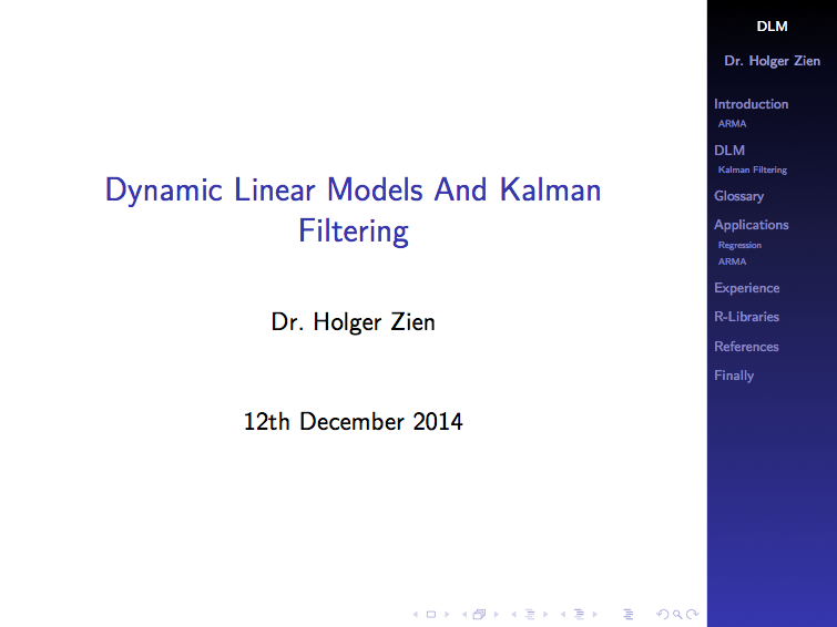
Dynamic Linear Models and Kalman Filtering
 |
| Download slides |
Nowadays, his challenges can be very different, sometimes only a few data points from a non-stationary process are available, and yet he is still expected to predict the future.
Dynamic linear models (dlm) can provide a remedy in those situations. In their simplest version a dlm links system and observational equations in the following way:
\[
y_t = F \theta_t + \nu_t\quad\mbox{observation eq. }\\
\theta_t = G \theta_{t-1} + \omega_t\quad\mbox{system eq.}
\] with \(\nu_t, \omega_t\) mutually independent random variables. A special case of dynamic linear models is the well known Kalman filter. In the more general case \(y_t\) and \(\theta_t\) are vectors and \(F_t, G_t\) are time variant matrices.
Holger explained that a dlm can principally be used for three purposes:
- Filtering: Estimate of the current value of the state/system variable.
- Smoothing: Estimate of past values of the state/system variable, i.e., estimating at time \(t\) given measurements up to time \(t' > t\).
- Forecasting: Forecasting future observations or values of the state/system variable.
Next Kölner R meeting
The next meeting is scheduled for 6 March 2015.Please get in touch if you would like to present and share your experience, or indeed if you have a request for a topic you would like to hear more about. For more details see also our Meetup page.
Thanks again to Bernd Weiß for hosting the event and Revolution Analytics for their sponsorship.
Bayesian
,
dlm
,
Julia
,
Kalman
,
Koelner R User
,
Kölner R Users
,
R
Measuring temperature with my Arduino
It is really getting colder in London - it is now about 5°C outside. The heating is on and I have got better at measuring the temperature at home as well. Or, so I believe.
Last week's approach of me guessing/feeling the temperature combined with an old thermometer was perhaps too simplistic and too unreliable. This week's attempt to measure the temperature with my Arduino might be a little OTT (over the top), but at least I am using the micro-controller again.

Yet, I have to overcome similar challenges again as last week. The Arduino with the temperature sensor (TMP36) should be a better device to measure the temperature than my thermometer, but it isn't perfect either and the readings will have some uncertainty as well. But, it will be easy to make frequent measurements and with a little trick I should be able to filter out the noise and get a much better view of the 'true' temperature.
The trick is Bayesian filtering, or as it turns out, a simplified Kalman filter (univariate, no control actions, no transition matrices).
I can't observe the temperature directly, I can only try to measure it. I think of this scenario as a series of Bayesian networks (or Hidden Markov Model). The hidden or latent variable is the 'true' temperature and the observable variable is the reading of my Arduino sensor.

I start with a prior guess of the Temperature at time \(k=0\), just like last week (note, here I will use \(x_k\) instead of \(\mu_k\)). My initial prior is \(N(x_0, \sigma_0^2)\). Now I predict the state (temperature) \(\hat{x}_1\) at the next time step. I expect the temperature to be largely unchanged and therefore my prediction is just \(\hat{x}_1 = x_0 + \varepsilon_P\) with \(\varepsilon_P \sim N(0, \sigma_P^2)\) describing the additional process variance going from one time step to the next. The process variance is independent from the uncertainty of \(x_0\), hence I can add them up and thus my prior for \(x_1\) is \(N(x_0, \sigma_0^2+\sigma_P^2)\).

The measurement of the temperature should reflect the 'true' temperature with some measurement uncertainty \(\sigma_M\). My prediction of the measurement is \(\hat{z}_1 = \hat{x}_1 + \varepsilon_M\) with \(\varepsilon_M \sim N(0, \sigma_M^2)\). The best estimator for \(\hat{z}_1\) is the actual measurement \(z_1\) and therefore the likelihood distribution of \(z_1|x_1\) is \(\,N(z_1, \sigma_M)\). Applying the formulas for Bayesian conjugates again gives the hyper-parameters for the posterior normal distribution \(x_1|\,z_1, x_0\), the temperature given the measurement and my prediction from the previous time step:
\[
x_1=\left.\left(\frac{x_0}{\sigma_0^2+\sigma_P^2} + \frac{z_1}{\sigma_M^2}\right)\right/\left(\frac{1}{\sigma_0^2+\sigma_P^2} + \frac{1}{\sigma_M^2}\right) \\
\sigma_1^2=\left(\frac{1}{\sigma_0^2+\sigma_P^2} + \frac{1}{\sigma_M^2}\right)^{-1}
\]With \(K_1 := \frac{\sigma_0^2+\sigma_P^2}{\sigma_M^2+\sigma_0^2+\sigma_P^2} \) this simplifies to:
\[
x_1 = K_1\, z_1 + (1 - K_1)\, x_0\\
\sigma_1^2 = (1 - K_1) (\sigma_0^2 + \sigma_P^2)
\]
This gives the simple iterative updating procedure (or Kalman filter):
\[
K_{k+1} = \frac{\sigma_k^2+\sigma_P^2}{\sigma_M^2+\sigma_k^2+\sigma_P^2} \\
\sigma_{k+1}^2 = (1 - K_{k+1}) (\sigma_k^2 + \sigma_P^2)\\
x_{k+1} = K_{k+1}\, z_{k+1} + (1 - K_{k+1})\, x_k
\]
In my code below I set the process variance to \(\sigma_P^2=0.01\) and the measurement variance to \(\sigma_M^2=0.5\), which led to a fairly stable reading of 21.5°C.

Changing the parameters \(\sigma_P\) and \(\sigma_M\) influence how quickly the filter reacts to changes. Here is an example where I briefly touch the temperature sensor with the above parameters. The time axis in those screen shots is about 6 seconds.

I have to do a bit more reading on the Kalman filter. It appears to be an immensely powerful tool to extract the signal from the noise. Well, it helped to put a man on the moon.
Last week's approach of me guessing/feeling the temperature combined with an old thermometer was perhaps too simplistic and too unreliable. This week's attempt to measure the temperature with my Arduino might be a little OTT (over the top), but at least I am using the micro-controller again.

Yet, I have to overcome similar challenges again as last week. The Arduino with the temperature sensor (TMP36) should be a better device to measure the temperature than my thermometer, but it isn't perfect either and the readings will have some uncertainty as well. But, it will be easy to make frequent measurements and with a little trick I should be able to filter out the noise and get a much better view of the 'true' temperature.
The trick is Bayesian filtering, or as it turns out, a simplified Kalman filter (univariate, no control actions, no transition matrices).
I can't observe the temperature directly, I can only try to measure it. I think of this scenario as a series of Bayesian networks (or Hidden Markov Model). The hidden or latent variable is the 'true' temperature and the observable variable is the reading of my Arduino sensor.

I start with a prior guess of the Temperature at time \(k=0\), just like last week (note, here I will use \(x_k\) instead of \(\mu_k\)). My initial prior is \(N(x_0, \sigma_0^2)\). Now I predict the state (temperature) \(\hat{x}_1\) at the next time step. I expect the temperature to be largely unchanged and therefore my prediction is just \(\hat{x}_1 = x_0 + \varepsilon_P\) with \(\varepsilon_P \sim N(0, \sigma_P^2)\) describing the additional process variance going from one time step to the next. The process variance is independent from the uncertainty of \(x_0\), hence I can add them up and thus my prior for \(x_1\) is \(N(x_0, \sigma_0^2+\sigma_P^2)\).

The measurement of the temperature should reflect the 'true' temperature with some measurement uncertainty \(\sigma_M\). My prediction of the measurement is \(\hat{z}_1 = \hat{x}_1 + \varepsilon_M\) with \(\varepsilon_M \sim N(0, \sigma_M^2)\). The best estimator for \(\hat{z}_1\) is the actual measurement \(z_1\) and therefore the likelihood distribution of \(z_1|x_1\) is \(\,N(z_1, \sigma_M)\). Applying the formulas for Bayesian conjugates again gives the hyper-parameters for the posterior normal distribution \(x_1|\,z_1, x_0\), the temperature given the measurement and my prediction from the previous time step:
\[
x_1=\left.\left(\frac{x_0}{\sigma_0^2+\sigma_P^2} + \frac{z_1}{\sigma_M^2}\right)\right/\left(\frac{1}{\sigma_0^2+\sigma_P^2} + \frac{1}{\sigma_M^2}\right) \\
\sigma_1^2=\left(\frac{1}{\sigma_0^2+\sigma_P^2} + \frac{1}{\sigma_M^2}\right)^{-1}
\]With \(K_1 := \frac{\sigma_0^2+\sigma_P^2}{\sigma_M^2+\sigma_0^2+\sigma_P^2} \) this simplifies to:
\[
x_1 = K_1\, z_1 + (1 - K_1)\, x_0\\
\sigma_1^2 = (1 - K_1) (\sigma_0^2 + \sigma_P^2)
\]
This gives the simple iterative updating procedure (or Kalman filter):
\[
K_{k+1} = \frac{\sigma_k^2+\sigma_P^2}{\sigma_M^2+\sigma_k^2+\sigma_P^2} \\
\sigma_{k+1}^2 = (1 - K_{k+1}) (\sigma_k^2 + \sigma_P^2)\\
x_{k+1} = K_{k+1}\, z_{k+1} + (1 - K_{k+1})\, x_k
\]
In my code below I set the process variance to \(\sigma_P^2=0.01\) and the measurement variance to \(\sigma_M^2=0.5\), which led to a fairly stable reading of 21.5°C.

Changing the parameters \(\sigma_P\) and \(\sigma_M\) influence how quickly the filter reacts to changes. Here is an example where I briefly touch the temperature sensor with the above parameters. The time axis in those screen shots is about 6 seconds.

I have to do a bit more reading on the Kalman filter. It appears to be an immensely powerful tool to extract the signal from the noise. Well, it helped to put a man on the moon.
Code
This is the Processing and Arduino code I used in this post. You may have to change the port number in line 28 to your own settings.
Arduino
,
Bayesian
,
Kalman
,
Processing
How cold is it? A Bayesian attempt to measure temperature
It is getting colder in London, yet it is still quite mild considering that it is late November. Well, indoors it still feels like 20°C (68°F) to me, but I have been told last week that I should switch on the heating.
Luckily I found an old thermometer to check. The thermometer showed 18°C. Is it really below 20°C?
The thermometer is quite old and I'm not sure that is works properly anymore. So, what shall I do now? Perhaps I should consider that both measurements are uncertain and try to combine them.
I believe that I can sense the temperature within ±3°C, while I think that the thermometer still works within ±2°C. Assuming that both measurements follow a Gaussian (Normal) distribution, with the uncertainties given as standard deviations, I can use Bayes' theorem to combine my hypothesis with the data. The posterior distribution will be Gaussian again with conjugated hyper-parameters:
\[
\mu=\left.\left(\frac{\mu_0}{\sigma_0^2} + \frac{\sum_{i=1}^n x_i}{s^2}\right)\right/\left(\frac{1}{\sigma_0^2} + \frac{n}{s^2}\right) \\
\sigma^2=\left(\frac{1}{\sigma_0^2} + \frac{n}{s^2}\right)^{-1}
\]With \(K := \frac{n\sigma_0^2}{s^2+n\sigma_0^2} \) this simplifies to:
\[
\mu = K\, \bar{x} + (1 - K)\, \mu_0 \mbox{, with } \bar{x}=\frac{1}{n}\sum_{i=1}^n x_i\\
\sigma = s \,\sqrt{K/n}
\]In my case I have: \(n=1,\; x_1=18^{\circ}C,\; s=2^{\circ}C,\; \mu_0=20^{\circ}C,\; \sigma_0=3^{\circ}C\).
Hence, the posterior distribution has parameters \(\mu=18.6^{\circ}C\) and \(\sigma=1.7^{\circ}C\). Thus, my best guess would be that is actually a little colder than I thought. One could argue that the probability that is below 20° is 80%.
Over the last five days my perception of the temperature didn't change, neither did the weather forecast, but the measurements showed: 18°C, 19°C, 17.5°C, 18°C, 18.5°C.
With that information the parameters update to \(\mu=18.3^{\circ}C\) and \(\sigma=0.9^{\circ}C\). I can't deny it any longer it has got colder. The probability that is below 20°C is now at 97% and the heating is on.

Without any prior knowledge I may have used a t-test to check the measurements. But here I believe that I have information about the thermometer and my own temperature sensing abilities which I don't want to ignore.
Luckily I found an old thermometer to check. The thermometer showed 18°C. Is it really below 20°C?
The thermometer is quite old and I'm not sure that is works properly anymore. So, what shall I do now? Perhaps I should consider that both measurements are uncertain and try to combine them.
I believe that I can sense the temperature within ±3°C, while I think that the thermometer still works within ±2°C. Assuming that both measurements follow a Gaussian (Normal) distribution, with the uncertainties given as standard deviations, I can use Bayes' theorem to combine my hypothesis with the data. The posterior distribution will be Gaussian again with conjugated hyper-parameters:
\[
\mu=\left.\left(\frac{\mu_0}{\sigma_0^2} + \frac{\sum_{i=1}^n x_i}{s^2}\right)\right/\left(\frac{1}{\sigma_0^2} + \frac{n}{s^2}\right) \\
\sigma^2=\left(\frac{1}{\sigma_0^2} + \frac{n}{s^2}\right)^{-1}
\]With \(K := \frac{n\sigma_0^2}{s^2+n\sigma_0^2} \) this simplifies to:
\[
\mu = K\, \bar{x} + (1 - K)\, \mu_0 \mbox{, with } \bar{x}=\frac{1}{n}\sum_{i=1}^n x_i\\
\sigma = s \,\sqrt{K/n}
\]In my case I have: \(n=1,\; x_1=18^{\circ}C,\; s=2^{\circ}C,\; \mu_0=20^{\circ}C,\; \sigma_0=3^{\circ}C\).
Hence, the posterior distribution has parameters \(\mu=18.6^{\circ}C\) and \(\sigma=1.7^{\circ}C\). Thus, my best guess would be that is actually a little colder than I thought. One could argue that the probability that is below 20° is 80%.
Over the last five days my perception of the temperature didn't change, neither did the weather forecast, but the measurements showed: 18°C, 19°C, 17.5°C, 18°C, 18.5°C.
With that information the parameters update to \(\mu=18.3^{\circ}C\) and \(\sigma=0.9^{\circ}C\). I can't deny it any longer it has got colder. The probability that is below 20°C is now at 97% and the heating is on.

Without any prior knowledge I may have used a t-test to check the measurements. But here I believe that I have information about the thermometer and my own temperature sensing abilities which I don't want to ignore.
R code
Session Info
R version 3.1.2 (2014-10-31)
Platform: x86_64-apple-darwin13.4.0 (64-bit)

locale:
[1] en_GB.UTF-8/en_GB.UTF-8/en_GB.UTF-8/C/en_GB.UTF-8/en_GB.UTF-8

attached base packages:
[1] stats     graphics  grDevices utils     datasets  methods
[7] base

other attached packages:
[1] BayesianFirstAid_0.1 rjags_3-14           coda_0.16-1
[4] lattice_0.20-29

loaded via a namespace (and not attached):
[1] grid_3.1.2 MASS_7.3-35 mnormt_1.5-1 stringr_0.6.2Hit and run. Think Bayes!
At the R in Insurance conference Arthur Charpentier gave a great keynote talk on Bayesian modelling in R. Bayes' theorem on conditional probabilities is strikingly simple, yet incredibly thought provoking. Here is an example from Daniel Kahneman to test your intuition. But first I have to start with Bayes' theorem.
\[
P(H \cap D) = P(H|D) \, P(D) = P(D|H) \, P(H)
\]
Or if I rearrange it:
\[
P(H|D) = \dfrac{P(D|H) \, P(H)}{P(D)}
\]
Imagine \(H\) is short for hypothesis and \(D\) is short for data, or evidence. Then Bayes' theorem states that the probability of a hypothesis given data is the same as the likelihood that we observe the data given the hypothesis, weighted by the prior belief of the hypothesis, normalised by the probability that we observe the data regardless of the hypothesis.
The tricky bit in real life is often to figure out what the hypothesis and data are.
What is here the data and what is here the hypothesis? Intuitively you may think that the proportion of Blue and Green cabs is the data at hand and the witness accusation that a Blue cab was involved in the accident is the hypothesis. However, after some thought I found the following assignment much more helpful, as then \(P(H|D)\) matches the above question:
\(H =\) Accident caused by Blue cab. \(D =\) Witness said the cab was Blue.
With this it is straightforward to get the probabilities of \(P(H)=15\%\) and \(P(D|H)=80\%\). But what is \(P(D)\)? Well, when would the witness say that the cab was Blue? Either, when the cab was Blue and so the witness is right, or when the cab was actually Green and the witness is incorrect. Thus, following the law of total probability:
$$\begin{align}
P(D) & = P(D|H) P(H) + P(D | \bar{H}) P(\bar{H})\\
& = 0.8 \cdot 0.15 + 0.2 \cdot 0.85 = 0.29
\end{align}$$Therefore I get \(P(H|D)=41\%\). Thus, even if the witness states that the cab involved in the accident was Blue, the probability of this being true is only \(41\%\).
An alternative way to think about this problem is via a Bayesian Network. The colour of the cab will influence the statement of the witness. In R I can specify such a network using the gRain package [2], which I discussed in an earlier post. Here I provide the distribution of the cabs and the conditional probabilities of the witness as an input. After I compile the network, I can again read off the probabilities that a Blue cab was involved, when the witness said so.

Bayes' theorem
Bayes' theorem states that given two events \(D\) and \(H\), the probability of \(D\) and \(H\) happening at the same time is the same as the probability of \(D\) occurring, given \(H\), weighted by the probability that \(H\) occurs; or the other way round. As a formula it can be written as:\[
P(H \cap D) = P(H|D) \, P(D) = P(D|H) \, P(H)
\]
Or if I rearrange it:
\[
P(H|D) = \dfrac{P(D|H) \, P(H)}{P(D)}
\]
Imagine \(H\) is short for hypothesis and \(D\) is short for data, or evidence. Then Bayes' theorem states that the probability of a hypothesis given data is the same as the likelihood that we observe the data given the hypothesis, weighted by the prior belief of the hypothesis, normalised by the probability that we observe the data regardless of the hypothesis.
The tricky bit in real life is often to figure out what the hypothesis and data are.
Hit and run accident
This example is taken from Daniel Kahneman's book Thinking, fast and slow [1].A cab was involved in a hit and run accident at night. Two cab companies, the Green and the Blue, operate in the city. 85% of the cabs in the city are Green and 15% are Blue. A witness identified the cab as Blue. The court tested the reliability of the witness under the same circumstances that existed on the night of the accident and concluded that the witness correctly identified each one of the two colours 80% of the time and failed 20% of the time.
What is the probability that the cab involved in the accident was Blue rather than Green knowing that this witness identified it as Blue?
What is here the data and what is here the hypothesis? Intuitively you may think that the proportion of Blue and Green cabs is the data at hand and the witness accusation that a Blue cab was involved in the accident is the hypothesis. However, after some thought I found the following assignment much more helpful, as then \(P(H|D)\) matches the above question:
\(H =\) Accident caused by Blue cab. \(D =\) Witness said the cab was Blue.
With this it is straightforward to get the probabilities of \(P(H)=15\%\) and \(P(D|H)=80\%\). But what is \(P(D)\)? Well, when would the witness say that the cab was Blue? Either, when the cab was Blue and so the witness is right, or when the cab was actually Green and the witness is incorrect. Thus, following the law of total probability:
$$\begin{align}
P(D) & = P(D|H) P(H) + P(D | \bar{H}) P(\bar{H})\\
& = 0.8 \cdot 0.15 + 0.2 \cdot 0.85 = 0.29
\end{align}$$Therefore I get \(P(H|D)=41\%\). Thus, even if the witness states that the cab involved in the accident was Blue, the probability of this being true is only \(41\%\).
An alternative way to think about this problem is via a Bayesian Network. The colour of the cab will influence the statement of the witness. In R I can specify such a network using the gRain package [2], which I discussed in an earlier post. Here I provide the distribution of the cabs and the conditional probabilities of the witness as an input. After I compile the network, I can again read off the probabilities that a Blue cab was involved, when the witness said so.


