Back from R/Finance in Chicago
I had a great time at the R/Finance conference in Chicago last Friday/Saturday. Some brief takeaways for me were:
From Emanuel Derman's talk: It is is important to distinguish between theories and models. Theories live in an abstract world and for a given set of axioms they can be proven right. However, models live in the real world, are build on simplifying assumptions and are only useful until experiments/data proves them wrong.
'Pornography is hard to define, but I know it when I see it.' Matt Dowle from h2o had the laughs on his side when he started his talk with this Justice Potter Stewart quote to illustrate the value of his
Bryan W. Lewis showed why inverting a matrix is tricky, particularly when it contains entries close to zero and what you can do about it.
Marius Hofert gave a stimulating talk on
Following a brief conversation with Dirk on
The audience seemed to have appreciated my talk on Communicating Risk. My chart of visualising profitability using a Whale Chart appeared to have resonated with a few.
Furthermore, I learned that the weather in Chicago is even more unstable than in London. After an amazing conference dinner at the Trump Tower, spending most of the time outside and admiring the sunset, we experienced a very cold and rainy Saturday. But then again, there is always time for a Jazz club and a drink. Talking about drinks, thanks to Q Ethan McCallum I had true American breakfast experience, including bottomless coffee.
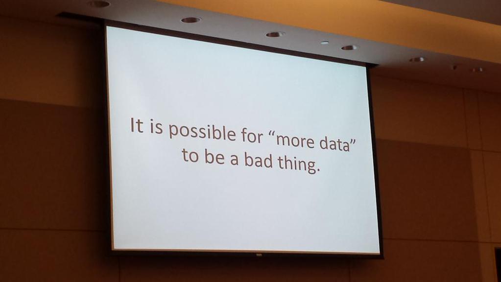
Yet, the last word should go to ShabbyChef, who took a photo of a slide during Louis Marascio's keynote and tweeted:

Amen.
From Emanuel Derman's talk: It is is important to distinguish between theories and models. Theories live in an abstract world and for a given set of axioms they can be proven right. However, models live in the real world, are build on simplifying assumptions and are only useful until experiments/data proves them wrong.
'Pornography is hard to define, but I know it when I see it.' Matt Dowle from h2o had the laughs on his side when he started his talk with this Justice Potter Stewart quote to illustrate the value of his
data.table package to its users.Bryan W. Lewis showed why inverting a matrix is tricky, particularly when it contains entries close to zero and what you can do about it.
Marius Hofert gave a stimulating talk on
simsalapar a package for parallel simulations, which I need to study in more detail.Following a brief conversation with Dirk on
drat I finally got the punch line of the package, but not so much the joke on drat as a fairly mild expression of anger or annoyance. I had never heard the expression in the UK. Perhaps drat is better explained as Dirk's R Archive Template?The audience seemed to have appreciated my talk on Communicating Risk. My chart of visualising profitability using a Whale Chart appeared to have resonated with a few.
Furthermore, I learned that the weather in Chicago is even more unstable than in London. After an amazing conference dinner at the Trump Tower, spending most of the time outside and admiring the sunset, we experienced a very cold and rainy Saturday. But then again, there is always time for a Jazz club and a drink. Talking about drinks, thanks to Q Ethan McCallum I had true American breakfast experience, including bottomless coffee.
Yet, the last word should go to ShabbyChef, who took a photo of a slide during Louis Marascio's keynote and tweeted:
Amen.
Conference
,
R
,
R in Finance
Communicating Risk at the Bay Area R User Group
I will be speaking at the Bay Area User Group meeting tonight about Communicating Risk. Anthony Goldbloom from Kaggle and Karim Chine from ElasticR will be there as well. The meeting will be at Microsoft in Mountain View.
Later this week I will give a similar presentation at the R in Finance conference in Chicago. Please get in touch if you are around and would like to share a coffee with me.
Later this week I will give a similar presentation at the R in Finance conference in Chicago. Please get in touch if you are around and would like to share a coffee with me.
Insurance
,
Presentations
,
R
Posterior predictive output with Stan
I continue my Stan experiments with another insurance example. Here I am particular interested in the posterior predictive distribution from only three data points. Or, to put it differently I have a customer of three years and I'd like to predict the expected claims cost for the next year to set or adjust the premium.
The example is taken from section 16.17 in Loss Models: From Data to Decisions [1]. Some time ago I used the same example to get my head around a Bayesian credibility model.
Suppose the claims likelihood distribution is believed to follow an exponential distribution for a given parameter \(\Theta\). The prior parameter distribution on \(\Theta\) is assumed to be a gamma distribution with parameters \(\alpha=4, \beta=1000\):
\[\begin{aligned}\Theta & \sim \mbox{Gamma}(\alpha, \beta)\\
\ell_i & \sim \mbox{Exp}(\Theta) , \; \forall i \in N
\end{aligned}\]In this case the predictive distribution is a Pareto II distribution with density \(f(x) = \frac{\alpha \beta^\alpha}{(x+\beta)^{\alpha+1}}\) and a mean of \(\frac{\beta}{\alpha-1}=\,\)333.33.
I have three independent observations, namely losses of $100, $950 and $450. The posterior predictive expected loss is $416.67 and can be derived analytical, as shown in my earlier post. Now let me reproduce the answer with Stan as well.
Implementing the model in Stan is straightforward and I follow the same steps as in my simple example of last week. However, here I am also interested in the posterior predictive distribution, hence I add a

The output shows a simulated predictive mean of $416.86, close to the analytical answer. I can also read out that the 75%ile of the posterior predictive distribution is a loss of $542 vs. $414 from the prior predictive. That means every four years I shouldn't be surprised to observe a loss in excess of $500. Further I note that 90% of losses are expected to be less than $950, or in other words the observation in my data may reflect the outcome of an event with a 1 in 10 return period.
Comparing the sampling output from Stan with the analytical output gives me some confidence that I am doing the 'right thing'.
The example is taken from section 16.17 in Loss Models: From Data to Decisions [1]. Some time ago I used the same example to get my head around a Bayesian credibility model.
Suppose the claims likelihood distribution is believed to follow an exponential distribution for a given parameter \(\Theta\). The prior parameter distribution on \(\Theta\) is assumed to be a gamma distribution with parameters \(\alpha=4, \beta=1000\):
\[\begin{aligned}\Theta & \sim \mbox{Gamma}(\alpha, \beta)\\
\ell_i & \sim \mbox{Exp}(\Theta) , \; \forall i \in N
\end{aligned}\]In this case the predictive distribution is a Pareto II distribution with density \(f(x) = \frac{\alpha \beta^\alpha}{(x+\beta)^{\alpha+1}}\) and a mean of \(\frac{\beta}{\alpha-1}=\,\)333.33.
I have three independent observations, namely losses of $100, $950 and $450. The posterior predictive expected loss is $416.67 and can be derived analytical, as shown in my earlier post. Now let me reproduce the answer with Stan as well.
Implementing the model in Stan is straightforward and I follow the same steps as in my simple example of last week. However, here I am also interested in the posterior predictive distribution, hence I add a
generated quantities code block. The output shows a simulated predictive mean of $416.86, close to the analytical answer. I can also read out that the 75%ile of the posterior predictive distribution is a loss of $542 vs. $414 from the prior predictive. That means every four years I shouldn't be surprised to observe a loss in excess of $500. Further I note that 90% of losses are expected to be less than $950, or in other words the observation in my data may reflect the outcome of an event with a 1 in 10 return period.
Comparing the sampling output from Stan with the analytical output gives me some confidence that I am doing the 'right thing'.
References
[1] Klugman, S. A., Panjer, H. H. & Willmot, G. E. (2004), Loss Models: From Data to Decisions, Wiley Series in Probability and Statistics.Session Info
R version 3.2.0 (2015-04-16)
Platform: x86_64-apple-darwin13.4.0 (64-bit)
Running under: OS X 10.10.3 (Yosemite)

locale:
[1] en_GB.UTF-8/en_GB.UTF-8/en_GB.UTF-8/C/en_GB.UTF-8/en_GB.UTF-8

attached base packages:
[1] stats graphics grDevices utils datasets methods base

other attached packages:
[1] lattice_0.20-31 actuar_1.1-8 rstan_2.6.0 inline_0.3.14
[5] Rcpp_0.11.6

loaded via a namespace (and not attached):
[1] tools_3.2.0  codetools_0.2-11 grid_3.2.0 stats4_3.2.0
Hello Stan!
In my previous post I discussed how Longley-Cook, an actuary at an insurance company in the 1950's, used Bayesian reasoning to estimate the probability for a mid-air collision of two planes.
Here I will use the same model to get started with Stan/RStan, a probabilistic programming language for Bayesian inference.
Last week my prior was given as a Beta distribution with parameters \(\alpha=1, \beta=1\) and the likelihood was assumed to be a Bernoulli distribution with parameter \(\theta\):
\[\begin{aligned}
\theta & \sim \mbox{Beta}(1, 1)\\
y_i & \sim \mbox{Bernoulli}(\theta), \;\forall i \in N
\end{aligned}\]For the previous five years no mid-air collision were observed, \(x=\{0, 0, 0, 0, 0\}\). That's my data.
In this case the posterior distributions can be derived analytically. The posterior hyper-parameters are \(\alpha'=\alpha + \sum_{i=1}^n x_i,\, \beta'=\beta + n - \sum_{i=1}^n x_i\) and with that I get the posterior parameter for the predictive distribution, which is a Bernoulli distribution again: \(\theta' = \alpha'/(\alpha'+\beta')=1/7\approx14.3\%\).
Still, I can use Stan and MCMC simulations to come to the same answers (of course I am using a sledgehammer here to crack a nut).
In the first code block the model is written in Stan's modelling language. The next section calls

Interested in the application of R in insurance? Join us at the 3rd R in Insurance conference in Amsterdam, 29 June 2015.
Here I will use the same model to get started with Stan/RStan, a probabilistic programming language for Bayesian inference.
Last week my prior was given as a Beta distribution with parameters \(\alpha=1, \beta=1\) and the likelihood was assumed to be a Bernoulli distribution with parameter \(\theta\):
\[\begin{aligned}
\theta & \sim \mbox{Beta}(1, 1)\\
y_i & \sim \mbox{Bernoulli}(\theta), \;\forall i \in N
\end{aligned}\]For the previous five years no mid-air collision were observed, \(x=\{0, 0, 0, 0, 0\}\). That's my data.
In this case the posterior distributions can be derived analytically. The posterior hyper-parameters are \(\alpha'=\alpha + \sum_{i=1}^n x_i,\, \beta'=\beta + n - \sum_{i=1}^n x_i\) and with that I get the posterior parameter for the predictive distribution, which is a Bernoulli distribution again: \(\theta' = \alpha'/(\alpha'+\beta')=1/7\approx14.3\%\).
Still, I can use Stan and MCMC simulations to come to the same answers (of course I am using a sledgehammer here to crack a nut).
In the first code block the model is written in Stan's modelling language. The next section calls
stan and finally the results can be analysed. The answers are very much the same as the analytical approach in my previous post.Interested in the application of R in insurance? Join us at the 3rd R in Insurance conference in Amsterdam, 29 June 2015.
Session Info
R version 3.2.0 (2015-04-16)
Platform: x86_64-apple-darwin13.4.0 (64-bit)
Running under: OS X 10.10.3 (Yosemite)

locale:
[1] en_GB.UTF-8/en_GB.UTF-8/en_GB.UTF-8/C/en_GB.UTF-8/en_GB.UTF-8

attached base packages:
[1] stats     graphics  grDevices utils     datasets  methods   base

other attached packages:
[1] rstan_2.6.0   inline_0.3.14 Rcpp_0.11.6

loaded via a namespace (and not attached):
[1] tools_3.2.0 codetools_0.2-11 stats4_3.2.0Predicting events, when they haven't happened yet
Suppose you have to predict the probabilities of events which haven't happened yet. How do you do this?
Here is an example from the 1950s when Longley-Cook, an actuary at an insurance company, was asked to price the risk for a mid-air collision of two planes, an event which as far as he knew hadn't happened before. The civilian airline industry was still very young, but rapidly growing and all Longely-Cook knew was that there were no collisions in the previous 5 years [1].
Where do you start?
Although the probability for a mid-air collision should be very low for any given plane, the probability for an event in a year will be higher.
Let's think of the years as a series of Bernoulli trials with unknown probability \(p\). That's a likelihood. If I start with an uninformed prior, such as a Beta(\(\alpha,\beta\)) with \(\alpha=1, \beta=1\) then I can use the concept of Bayesian conjugates to update my prior believe.
In this case the posterior parameter distribution is Beta again with hyper-parameters \(\alpha'=\alpha + \sum_{i=1}^n x_i,\, \beta'=\beta + n - \sum_{i=1}^n x_i\), where \(x_i=1\) if the event occurred, or 0 otherwise and \(n\) is the number of years.
Thus, the updated parameters are \(\alpha'=1, \beta'=6\), with a posterior predictive mean of \(\alpha'/(\alpha'+\beta')=1/7\). That is a 14.3% chance for a mid-air collision in the next year with a 95% confidence interval of [0, 39%]. Or, in other words, if I round 39% to 40%, a return period of 2.5 years (1/0.4), i.e. up to 4 incidents in 10 years should be allowed for. That's what Longley-Cook predicted.
Tragically, 128 people died over the Grand Canyon in 1956, and 4 years after that, 134 people died over New York City.
Wikipedia lists 51 notable civilian mid-air collisions since 1922, including helicopters and space crafts. Since 1955 there were 11 incidents that had more than 100 fatalities, the last one in 2006.
So, what would this mean to Mr. Longley-Cook today? Well, first of all that his prediction wasn't too bad at all. Perhaps, he would set the probability at (1+11)/((1+11)+(1+60-11)\(\approx\)20% today. He may have argued that 2 x 20% = 40% of the average plane value should be included in the world wide premium for airline hull to cover mid-air collisions.

Interested in the application of R in insurance? Join us at the 3rd R in Insurance conference in Amsterdam, 29 June 2015.
Here is an example from the 1950s when Longley-Cook, an actuary at an insurance company, was asked to price the risk for a mid-air collision of two planes, an event which as far as he knew hadn't happened before. The civilian airline industry was still very young, but rapidly growing and all Longely-Cook knew was that there were no collisions in the previous 5 years [1].
Where do you start?
Although the probability for a mid-air collision should be very low for any given plane, the probability for an event in a year will be higher.
Let's think of the years as a series of Bernoulli trials with unknown probability \(p\). That's a likelihood. If I start with an uninformed prior, such as a Beta(\(\alpha,\beta\)) with \(\alpha=1, \beta=1\) then I can use the concept of Bayesian conjugates to update my prior believe.
In this case the posterior parameter distribution is Beta again with hyper-parameters \(\alpha'=\alpha + \sum_{i=1}^n x_i,\, \beta'=\beta + n - \sum_{i=1}^n x_i\), where \(x_i=1\) if the event occurred, or 0 otherwise and \(n\) is the number of years.
Thus, the updated parameters are \(\alpha'=1, \beta'=6\), with a posterior predictive mean of \(\alpha'/(\alpha'+\beta')=1/7\). That is a 14.3% chance for a mid-air collision in the next year with a 95% confidence interval of [0, 39%]. Or, in other words, if I round 39% to 40%, a return period of 2.5 years (1/0.4), i.e. up to 4 incidents in 10 years should be allowed for. That's what Longley-Cook predicted.
Tragically, 128 people died over the Grand Canyon in 1956, and 4 years after that, 134 people died over New York City.
Wikipedia lists 51 notable civilian mid-air collisions since 1922, including helicopters and space crafts. Since 1955 there were 11 incidents that had more than 100 fatalities, the last one in 2006.
So, what would this mean to Mr. Longley-Cook today? Well, first of all that his prediction wasn't too bad at all. Perhaps, he would set the probability at (1+11)/((1+11)+(1+60-11)\(\approx\)20% today. He may have argued that 2 x 20% = 40% of the average plane value should be included in the world wide premium for airline hull to cover mid-air collisions.
R code
Interested in the application of R in insurance? Join us at the 3rd R in Insurance conference in Amsterdam, 29 June 2015.
References
[1] Computational Actuarial Science with R, Edited by Arthur Charpentier, Chapman and Hall/CRC Reference - 656 PagesSession Info
R version 3.2.0 (2015-04-16)
Platform: x86_64-apple-darwin13.4.0 (64-bit)
Running under: OS X 10.10.3 (Yosemite)

locale:
[1] en_GB.UTF-8/en_GB.UTF-8/en_GB.UTF-8/C/en_GB.UTF-8/en_GB.UTF-8

attached base packages:
[1] stats     graphics  grDevices utils     datasets  methods
[7] base

other attached packages:
[1] XML_3.98-1.1

loaded via a namespace (and not attached):
[1] tools_3.2.0R in Insurance 2015 Conference Programme
The programme for the 3rd R in Insurance conference is on-line. The event will take place on 29 June 2015 at the University of Amsterdam. Time to register now.

Special thanks to our sponsors, without whom the conference wouldn't be possible:
CYBAEA, RStudio, APPLIED AI, Milliman, QBE Re, AEGON, Delta Lloyd Amsterdam , Deloitte.
You find impressions from the previous events on www.rininsurance.com.
We hope to see you in Amsterdam!
Special thanks to our sponsors, without whom the conference wouldn't be possible:
CYBAEA, RStudio, APPLIED AI, Milliman, QBE Re, AEGON, Delta Lloyd Amsterdam , Deloitte.
You find impressions from the previous events on www.rininsurance.com.
We hope to see you in Amsterdam!
Combining several lattice charts into one
Last week I mentioned the
Here is minimal example from the help file of

In my next example I am using data from Eurostat, the statistical office of the European Union, showing the use of public transport in four countries. The data can be accessed directly in R via the eurostat package; see also the package vignette.

Here I have two
grid.arrange function of the gridExtra package that allows me to combine graphical grid objects onto one page. The latticeExtra package provides another elegant solution for trellis (lattice) plots: the function c.trellis() or just c() combines the panels of multiple trellis objects into one. Here is minimal example from the help file of
c.trellis:library(latticeExtra)
## Combine different types of plots.
c(wireframe(volcano), contourplot(volcano))

In my next example I am using data from Eurostat, the statistical office of the European Union, showing the use of public transport in four countries. The data can be accessed directly in R via the eurostat package; see also the package vignette.

Here I have two
xyplot objects that I combine into one chart using a named vector. I know this is not the best way to present the data, but that is not the point here. Naming the elements in c() adds those names also into the panel strip. Very handy indeed!Session Info
R version 3.1.3 (2015-03-09)
Platform: x86_64-apple-darwin13.4.0 (64-bit)
Running under: OS X 10.10.3 (Yosemite)

locale:
[1] en_GB.UTF-8/en_GB.UTF-8/en_GB.UTF-8/C/en_GB.UTF-8/en_GB.UTF-8

attached base packages:
[1] stats     graphics  grDevices utils     datasets  methods
[7] base

other attached packages:
[1] latticeExtra_0.6-26 lattice_0.20-31     RColorBrewer_1.1-2
[4] eurostat_1.0.16

loaded via a namespace (and not attached):
[1] grid_3.1.3     plyr_1.8.1     Rcpp_0.11.5    reshape2_1.4.1
[5] stringi_0.4-1  stringr_0.6.2  tidyr_0.2.0    tools_3.1.3
c.trellis
,
eurostat
,
latticeExtra
,
R


