The reshape function

The other day I wrote about the R functions by, apply and friends, which allow me to operate on subsets of data. All those functions work nicely, if the data is given in the right format. More often than not it isn't and I have to reshape the data beforehand. Thus, time to discuss the reshape function. I will focus on the reshape function in base R, and not the package of the same name.

I use Fischer's iris data set again, as it is readily available after starting R. The iris data set has 150 observation and the first 6 rows look like this:

head(iris)
  Sepal.Length Sepal.Width Petal.Length Petal.Width Species
1          5.1         3.5          1.4         0.2  setosa
2          4.9         3.0          1.4         0.2  setosa
3          4.7         3.2          1.3         0.2  setosa
4          4.6         3.1          1.5         0.2  setosa
5          5.0         3.6          1.4         0.2  setosa
6          5.4         3.9          1.7         0.4  setosa

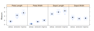
I would like to create a box whisker plot, showing the measurements of the observations for each of the species, as in the chart below.

I know, that if I had all measurements in one column and the dimension in another column, I could produce a graph like this in one line with lattice.

library(lattice)
bwplot(Measurement ~ Species | Dimension, data=reshaped.iris)

reshaped.iris <- reshape(iris, varying=1:4, v.names="Measurement", 
                         timevar="Dimension", times=names(iris)[1:4], 
                         idvar="Measure ID", direction="long") 

head(reshaped.iris)
               Species    Dimension Measurement Measure ID
1.Sepal.Length  setosa Sepal.Length         5.1          1
2.Sepal.Length  setosa Sepal.Length         4.9          2
3.Sepal.Length  setosa Sepal.Length         4.7          3
4.Sepal.Length  setosa Sepal.Length         4.6          4
5.Sepal.Length  setosa Sepal.Length         5.0          5
6.Sepal.Length  setosa Sepal.Length         5.4          6

In my next example I would like the measurements of length and width in separate columns and capture the flower part in a new variable, so I can create scatterplots of length against width. Tweaking the reshape statement slightly gives me:

reshaped.iris.sp <- reshape(iris, varying=list(c(1,3),c(2,4)),
                            v.names=c("Length", "Width"), 
                            timevar="Part", times=c("Sepal", "Petal"),
                            idvar="Measure ID", direction="long")

head(reshaped.iris.sp)
        Species  Part Length Width Measure ID
1.Sepal  setosa Sepal    5.1   3.5          1
2.Sepal  setosa Sepal    4.9   3.0          2
3.Sepal  setosa Sepal    4.7   3.2          3
4.Sepal  setosa Sepal    4.6   3.1          4
5.Sepal  setosa Sepal    5.0   3.6          5
6.Sepal  setosa Sepal    5.4   3.9          6

xyplot(Length ~  Width | Species, groups=Part, 
       data=reshaped.iris.sp, auto.key=list(space="right"))

xyplot(Length ~  Width | Part, groups=Species, 
       data=reshaped.iris.sp, auto.key=list(space="right"))

I think, the charts illustrate quite nicely why the iris data set has become a typical test case for many classification techniques in machine learning.