Notes from the Kölner R meeting, 12 December 2014
Last week's Cologne R user group meeting was the best attended so far, and it was a remarkable event - I believe not a single line of R code was shown. Still, it was an R user group meeting with two excellent talks, and you will understand shortly why not much R code needed to be displayed.
Hans Werner Borchers joined us from Mannheim to give an introduction to Julia for R users. Julia is a high-level, high-performance dynamic programming language for technical computing. The language has gained some considerable traction over the last two years and it was great to get an overview from a familiar perspective.
Interestingly, as Hans Werner pointed out, Julia is by far not the only new language around the block. Indeed, over the last decade nearly every year saw the announcement of a new language. Also big tech companies such as Microsoft, Google, Mozilla and Apple are trying to push their own programming languages: F# (2005), Go (2009), Rust (2010) and Swift (2014) respectively.
Over the more recent years we notice a movement towards the use of LLVM (Low Level Virtual Machine), on which Julia is based as well and which makes it fast. The just in time compilation demands a little mind shift if you come from R, where the mantra for speed is: vectorise - remove all for-loops. Well, the opposite is true for Julia, because your code will be compiled. For-loops are much easier to understand for the underlying compiler. Hans Werner's slides provide some good examples to get you started and pointers to further resources.
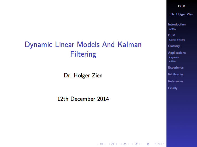
Forecasting time series was the topic of Holger Zien's talk. Holger gained his first experience with time series during his PhD, when he worked with experimental sensor data. That meant he had lots of data, which could often be regarded stationary as well.
Nowadays, his challenges can be very different, sometimes only a few data points from a non-stationary process are available, and yet he is still expected to predict the future.
Dynamic linear models (dlm) can provide a remedy in those situations. In their simplest version a dlm links system and observational equations in the following way:
\[
y_t = F \theta_t + \nu_t\quad\mbox{observation eq. }\\
\theta_t = G \theta_{t-1} + \omega_t\quad\mbox{system eq.}
\] with \(\nu_t, \omega_t\) mutually independent random variables. A special case of dynamic linear models is the well known Kalman filter. In the more general case \(y_t\) and \(\theta_t\) are vectors and \(F_t, G_t\) are time variant matrices.
Holger explained that a dlm can principally be used for three purposes:
Please get in touch if you would like to present and share your experience, or indeed if you have a request for a topic you would like to hear more about. For more details see also our Meetup page.
Thanks again to Bernd Weiß for hosting the event and Revolution Analytics for their sponsorship.
Introduction to Julia for R Users
 |
| Download slides |
Interestingly, as Hans Werner pointed out, Julia is by far not the only new language around the block. Indeed, over the last decade nearly every year saw the announcement of a new language. Also big tech companies such as Microsoft, Google, Mozilla and Apple are trying to push their own programming languages: F# (2005), Go (2009), Rust (2010) and Swift (2014) respectively.
Over the more recent years we notice a movement towards the use of LLVM (Low Level Virtual Machine), on which Julia is based as well and which makes it fast. The just in time compilation demands a little mind shift if you come from R, where the mantra for speed is: vectorise - remove all for-loops. Well, the opposite is true for Julia, because your code will be compiled. For-loops are much easier to understand for the underlying compiler. Hans Werner's slides provide some good examples to get you started and pointers to further resources.
Dynamic Linear Models and Kalman Filtering
 |
| Download slides |
Nowadays, his challenges can be very different, sometimes only a few data points from a non-stationary process are available, and yet he is still expected to predict the future.
Dynamic linear models (dlm) can provide a remedy in those situations. In their simplest version a dlm links system and observational equations in the following way:
\[
y_t = F \theta_t + \nu_t\quad\mbox{observation eq. }\\
\theta_t = G \theta_{t-1} + \omega_t\quad\mbox{system eq.}
\] with \(\nu_t, \omega_t\) mutually independent random variables. A special case of dynamic linear models is the well known Kalman filter. In the more general case \(y_t\) and \(\theta_t\) are vectors and \(F_t, G_t\) are time variant matrices.
Holger explained that a dlm can principally be used for three purposes:
- Filtering: Estimate of the current value of the state/system variable.
- Smoothing: Estimate of past values of the state/system variable, i.e., estimating at time \(t\) given measurements up to time \(t' > t\).
- Forecasting: Forecasting future observations or values of the state/system variable.
Next Kölner R meeting
The next meeting is scheduled for 6 March 2015.Please get in touch if you would like to present and share your experience, or indeed if you have a request for a topic you would like to hear more about. For more details see also our Meetup page.
Thanks again to Bernd Weiß for hosting the event and Revolution Analytics for their sponsorship.
Bayesian
,
dlm
,
Julia
,
Kalman
,
Koelner R User
,
Kölner R Users
,
R
Next Kölner R User Meeting: Friday, 12 December 2014

The next Cologne R user group meeting is scheduled for this Friday, 12 December 2014.
We have an exciting agenda with two talks on Julia and Dynamic Linear Models:
Introduction to Julia for R Users
Hans Werner BorchersJulia is a high-performance dynamic programming language for scientific computing, with a syntax that is familiar to users of other technical computing environments (Matlab, Python, R, etc.). It provides a sophisticated compiler, high performance with numerical accuracy, and extensive mathematical function libraries.
Some of the highlights of Julia are an implementation of automated differentiation, an optimisation modelling language, also integrating some of the optimisation solvers available from the COIN-OR project, and user-contributed packages for time series, statistics and machine learning, or operations research.
Dynamic Linear Models and Kalman Filtering
Holger ZienOne of the problems most commonly presented to everybody working in statistics is forecasting time series. The textbook answer is to fit an ARMA model to the data and to use the model for prediction. This approach works well for long and stationary time series. However, often the actual time series one is given to analyse are more complicated. They are ridiculously short and clearly non-stationary. Dynamic Linear Models (DLM) and Kalman Filtering go one step beyond ARMA models and may be applied to these more complicated data. I will give a brief introduction into their mathematical background and will talk about my experience using them in practice.
Drinks and Networking
The event will be followed by drinks and schnitzel at the Lux.For further details visit our KölnRUG Meetup site. Please sign up if you would like to come along. Notes from past meetings are available here.
The organisers, Bernd Weiß and Markus Gesmann, gratefully acknowledge the sponsorship of Revolution Analytics, who support the Cologne R user group as part of their vector programme.
View Larger Map
Measuring temperature with my Arduino
It is really getting colder in London - it is now about 5°C outside. The heating is on and I have got better at measuring the temperature at home as well. Or, so I believe.
Last week's approach of me guessing/feeling the temperature combined with an old thermometer was perhaps too simplistic and too unreliable. This week's attempt to measure the temperature with my Arduino might be a little OTT (over the top), but at least I am using the micro-controller again.

Yet, I have to overcome similar challenges again as last week. The Arduino with the temperature sensor (TMP36) should be a better device to measure the temperature than my thermometer, but it isn't perfect either and the readings will have some uncertainty as well. But, it will be easy to make frequent measurements and with a little trick I should be able to filter out the noise and get a much better view of the 'true' temperature.
The trick is Bayesian filtering, or as it turns out, a simplified Kalman filter (univariate, no control actions, no transition matrices).
I can't observe the temperature directly, I can only try to measure it. I think of this scenario as a series of Bayesian networks (or Hidden Markov Model). The hidden or latent variable is the 'true' temperature and the observable variable is the reading of my Arduino sensor.

I start with a prior guess of the Temperature at time \(k=0\), just like last week (note, here I will use \(x_k\) instead of \(\mu_k\)). My initial prior is \(N(x_0, \sigma_0^2)\). Now I predict the state (temperature) \(\hat{x}_1\) at the next time step. I expect the temperature to be largely unchanged and therefore my prediction is just \(\hat{x}_1 = x_0 + \varepsilon_P\) with \(\varepsilon_P \sim N(0, \sigma_P^2)\) describing the additional process variance going from one time step to the next. The process variance is independent from the uncertainty of \(x_0\), hence I can add them up and thus my prior for \(x_1\) is \(N(x_0, \sigma_0^2+\sigma_P^2)\).

The measurement of the temperature should reflect the 'true' temperature with some measurement uncertainty \(\sigma_M\). My prediction of the measurement is \(\hat{z}_1 = \hat{x}_1 + \varepsilon_M\) with \(\varepsilon_M \sim N(0, \sigma_M^2)\). The best estimator for \(\hat{z}_1\) is the actual measurement \(z_1\) and therefore the likelihood distribution of \(z_1|x_1\) is \(\,N(z_1, \sigma_M)\). Applying the formulas for Bayesian conjugates again gives the hyper-parameters for the posterior normal distribution \(x_1|\,z_1, x_0\), the temperature given the measurement and my prediction from the previous time step:
\[
x_1=\left.\left(\frac{x_0}{\sigma_0^2+\sigma_P^2} + \frac{z_1}{\sigma_M^2}\right)\right/\left(\frac{1}{\sigma_0^2+\sigma_P^2} + \frac{1}{\sigma_M^2}\right) \\
\sigma_1^2=\left(\frac{1}{\sigma_0^2+\sigma_P^2} + \frac{1}{\sigma_M^2}\right)^{-1}
\]With \(K_1 := \frac{\sigma_0^2+\sigma_P^2}{\sigma_M^2+\sigma_0^2+\sigma_P^2} \) this simplifies to:
\[
x_1 = K_1\, z_1 + (1 - K_1)\, x_0\\
\sigma_1^2 = (1 - K_1) (\sigma_0^2 + \sigma_P^2)
\]
This gives the simple iterative updating procedure (or Kalman filter):
\[
K_{k+1} = \frac{\sigma_k^2+\sigma_P^2}{\sigma_M^2+\sigma_k^2+\sigma_P^2} \\
\sigma_{k+1}^2 = (1 - K_{k+1}) (\sigma_k^2 + \sigma_P^2)\\
x_{k+1} = K_{k+1}\, z_{k+1} + (1 - K_{k+1})\, x_k
\]
In my code below I set the process variance to \(\sigma_P^2=0.01\) and the measurement variance to \(\sigma_M^2=0.5\), which led to a fairly stable reading of 21.5°C.

Changing the parameters \(\sigma_P\) and \(\sigma_M\) influence how quickly the filter reacts to changes. Here is an example where I briefly touch the temperature sensor with the above parameters. The time axis in those screen shots is about 6 seconds.

I have to do a bit more reading on the Kalman filter. It appears to be an immensely powerful tool to extract the signal from the noise. Well, it helped to put a man on the moon.
Last week's approach of me guessing/feeling the temperature combined with an old thermometer was perhaps too simplistic and too unreliable. This week's attempt to measure the temperature with my Arduino might be a little OTT (over the top), but at least I am using the micro-controller again.

Yet, I have to overcome similar challenges again as last week. The Arduino with the temperature sensor (TMP36) should be a better device to measure the temperature than my thermometer, but it isn't perfect either and the readings will have some uncertainty as well. But, it will be easy to make frequent measurements and with a little trick I should be able to filter out the noise and get a much better view of the 'true' temperature.
The trick is Bayesian filtering, or as it turns out, a simplified Kalman filter (univariate, no control actions, no transition matrices).
I can't observe the temperature directly, I can only try to measure it. I think of this scenario as a series of Bayesian networks (or Hidden Markov Model). The hidden or latent variable is the 'true' temperature and the observable variable is the reading of my Arduino sensor.

I start with a prior guess of the Temperature at time \(k=0\), just like last week (note, here I will use \(x_k\) instead of \(\mu_k\)). My initial prior is \(N(x_0, \sigma_0^2)\). Now I predict the state (temperature) \(\hat{x}_1\) at the next time step. I expect the temperature to be largely unchanged and therefore my prediction is just \(\hat{x}_1 = x_0 + \varepsilon_P\) with \(\varepsilon_P \sim N(0, \sigma_P^2)\) describing the additional process variance going from one time step to the next. The process variance is independent from the uncertainty of \(x_0\), hence I can add them up and thus my prior for \(x_1\) is \(N(x_0, \sigma_0^2+\sigma_P^2)\).

The measurement of the temperature should reflect the 'true' temperature with some measurement uncertainty \(\sigma_M\). My prediction of the measurement is \(\hat{z}_1 = \hat{x}_1 + \varepsilon_M\) with \(\varepsilon_M \sim N(0, \sigma_M^2)\). The best estimator for \(\hat{z}_1\) is the actual measurement \(z_1\) and therefore the likelihood distribution of \(z_1|x_1\) is \(\,N(z_1, \sigma_M)\). Applying the formulas for Bayesian conjugates again gives the hyper-parameters for the posterior normal distribution \(x_1|\,z_1, x_0\), the temperature given the measurement and my prediction from the previous time step:
\[
x_1=\left.\left(\frac{x_0}{\sigma_0^2+\sigma_P^2} + \frac{z_1}{\sigma_M^2}\right)\right/\left(\frac{1}{\sigma_0^2+\sigma_P^2} + \frac{1}{\sigma_M^2}\right) \\
\sigma_1^2=\left(\frac{1}{\sigma_0^2+\sigma_P^2} + \frac{1}{\sigma_M^2}\right)^{-1}
\]With \(K_1 := \frac{\sigma_0^2+\sigma_P^2}{\sigma_M^2+\sigma_0^2+\sigma_P^2} \) this simplifies to:
\[
x_1 = K_1\, z_1 + (1 - K_1)\, x_0\\
\sigma_1^2 = (1 - K_1) (\sigma_0^2 + \sigma_P^2)
\]
This gives the simple iterative updating procedure (or Kalman filter):
\[
K_{k+1} = \frac{\sigma_k^2+\sigma_P^2}{\sigma_M^2+\sigma_k^2+\sigma_P^2} \\
\sigma_{k+1}^2 = (1 - K_{k+1}) (\sigma_k^2 + \sigma_P^2)\\
x_{k+1} = K_{k+1}\, z_{k+1} + (1 - K_{k+1})\, x_k
\]
In my code below I set the process variance to \(\sigma_P^2=0.01\) and the measurement variance to \(\sigma_M^2=0.5\), which led to a fairly stable reading of 21.5°C.

Changing the parameters \(\sigma_P\) and \(\sigma_M\) influence how quickly the filter reacts to changes. Here is an example where I briefly touch the temperature sensor with the above parameters. The time axis in those screen shots is about 6 seconds.

I have to do a bit more reading on the Kalman filter. It appears to be an immensely powerful tool to extract the signal from the noise. Well, it helped to put a man on the moon.
Code
This is the Processing and Arduino code I used in this post. You may have to change the port number in line 28 to your own settings.
Arduino
,
Bayesian
,
Kalman
,
Processing
How cold is it? A Bayesian attempt to measure temperature
It is getting colder in London, yet it is still quite mild considering that it is late November. Well, indoors it still feels like 20°C (68°F) to me, but I have been told last week that I should switch on the heating.
Luckily I found an old thermometer to check. The thermometer showed 18°C. Is it really below 20°C?
The thermometer is quite old and I'm not sure that is works properly anymore. So, what shall I do now? Perhaps I should consider that both measurements are uncertain and try to combine them.
I believe that I can sense the temperature within ±3°C, while I think that the thermometer still works within ±2°C. Assuming that both measurements follow a Gaussian (Normal) distribution, with the uncertainties given as standard deviations, I can use Bayes' theorem to combine my hypothesis with the data. The posterior distribution will be Gaussian again with conjugated hyper-parameters:
\[
\mu=\left.\left(\frac{\mu_0}{\sigma_0^2} + \frac{\sum_{i=1}^n x_i}{s^2}\right)\right/\left(\frac{1}{\sigma_0^2} + \frac{n}{s^2}\right) \\
\sigma^2=\left(\frac{1}{\sigma_0^2} + \frac{n}{s^2}\right)^{-1}
\]With \(K := \frac{n\sigma_0^2}{s^2+n\sigma_0^2} \) this simplifies to:
\[
\mu = K\, \bar{x} + (1 - K)\, \mu_0 \mbox{, with } \bar{x}=\frac{1}{n}\sum_{i=1}^n x_i\\
\sigma = s \,\sqrt{K/n}
\]In my case I have: \(n=1,\; x_1=18^{\circ}C,\; s=2^{\circ}C,\; \mu_0=20^{\circ}C,\; \sigma_0=3^{\circ}C\).
Hence, the posterior distribution has parameters \(\mu=18.6^{\circ}C\) and \(\sigma=1.7^{\circ}C\). Thus, my best guess would be that is actually a little colder than I thought. One could argue that the probability that is below 20° is 80%.
Over the last five days my perception of the temperature didn't change, neither did the weather forecast, but the measurements showed: 18°C, 19°C, 17.5°C, 18°C, 18.5°C.
With that information the parameters update to \(\mu=18.3^{\circ}C\) and \(\sigma=0.9^{\circ}C\). I can't deny it any longer it has got colder. The probability that is below 20°C is now at 97% and the heating is on.

Without any prior knowledge I may have used a t-test to check the measurements. But here I believe that I have information about the thermometer and my own temperature sensing abilities which I don't want to ignore.
Luckily I found an old thermometer to check. The thermometer showed 18°C. Is it really below 20°C?
The thermometer is quite old and I'm not sure that is works properly anymore. So, what shall I do now? Perhaps I should consider that both measurements are uncertain and try to combine them.
I believe that I can sense the temperature within ±3°C, while I think that the thermometer still works within ±2°C. Assuming that both measurements follow a Gaussian (Normal) distribution, with the uncertainties given as standard deviations, I can use Bayes' theorem to combine my hypothesis with the data. The posterior distribution will be Gaussian again with conjugated hyper-parameters:
\[
\mu=\left.\left(\frac{\mu_0}{\sigma_0^2} + \frac{\sum_{i=1}^n x_i}{s^2}\right)\right/\left(\frac{1}{\sigma_0^2} + \frac{n}{s^2}\right) \\
\sigma^2=\left(\frac{1}{\sigma_0^2} + \frac{n}{s^2}\right)^{-1}
\]With \(K := \frac{n\sigma_0^2}{s^2+n\sigma_0^2} \) this simplifies to:
\[
\mu = K\, \bar{x} + (1 - K)\, \mu_0 \mbox{, with } \bar{x}=\frac{1}{n}\sum_{i=1}^n x_i\\
\sigma = s \,\sqrt{K/n}
\]In my case I have: \(n=1,\; x_1=18^{\circ}C,\; s=2^{\circ}C,\; \mu_0=20^{\circ}C,\; \sigma_0=3^{\circ}C\).
Hence, the posterior distribution has parameters \(\mu=18.6^{\circ}C\) and \(\sigma=1.7^{\circ}C\). Thus, my best guess would be that is actually a little colder than I thought. One could argue that the probability that is below 20° is 80%.
Over the last five days my perception of the temperature didn't change, neither did the weather forecast, but the measurements showed: 18°C, 19°C, 17.5°C, 18°C, 18.5°C.
With that information the parameters update to \(\mu=18.3^{\circ}C\) and \(\sigma=0.9^{\circ}C\). I can't deny it any longer it has got colder. The probability that is below 20°C is now at 97% and the heating is on.

Without any prior knowledge I may have used a t-test to check the measurements. But here I believe that I have information about the thermometer and my own temperature sensing abilities which I don't want to ignore.
R code
Session Info
R version 3.1.2 (2014-10-31)
Platform: x86_64-apple-darwin13.4.0 (64-bit)

locale:
[1] en_GB.UTF-8/en_GB.UTF-8/en_GB.UTF-8/C/en_GB.UTF-8/en_GB.UTF-8

attached base packages:
[1] stats     graphics  grDevices utils     datasets  methods
[7] base

other attached packages:
[1] BayesianFirstAid_0.1 rjags_3-14           coda_0.16-1
[4] lattice_0.20-29

loaded via a namespace (and not attached):
[1] grid_3.1.2 MASS_7.3-35 mnormt_1.5-1 stringr_0.6.2First steps with ChainLadder: Import triangle from Excel into R
Taking the first step is often the hardest: getting data from Excel into R.
Suppose you would like to use the

How do you get the triangle into R and execute a reserving function, such as
Well, there are many ways to do this and the ChainLadder package vignette, as well as the R manual on Data Import/Export has all of the details, but here is a quick and dirty solution using a CSV-file.
Open a new Excel workbook and copy your triangle into cell A1, with the first column being the accident or origin period and the first row describing the development period or age. You find an example CSV-file on GitHub.
Make sure that your triangle has no formatting, such a commas to separate thousands, as Excel will save those cell as characters. Now open R and go through the following commands:
To copy the full triangle back into Excel you can use the clipboard:
Go back to Excel and hit <Ctrl> + V on your keyboard to paste the data into R.
For more details see the package vignette and Dan's post on pasting triangles from Excel into R via the clipboard.
If you are after a thorough overview of R in insurance take a look at the book Computational Actuarial Science with R.
Finally, join the Special Interest Group on using R in actuarial science and insurance to share your questions and answers.
Suppose you would like to use the
ChainLadder package to forecast future claims payments for a run-off triangle that you have stored in Excel.
How do you get the triangle into R and execute a reserving function, such as
MackChainLadder?Well, there are many ways to do this and the ChainLadder package vignette, as well as the R manual on Data Import/Export has all of the details, but here is a quick and dirty solution using a CSV-file.
Open a new Excel workbook and copy your triangle into cell A1, with the first column being the accident or origin period and the first row describing the development period or age. You find an example CSV-file on GitHub.
Make sure that your triangle has no formatting, such a commas to separate thousands, as Excel will save those cell as characters. Now open R and go through the following commands:
# The first command will open a window and
# ask you to select your CSV-file
myCSVfile <- file.choose()
# Read file into R
dat <- read.csv(file=myCSVfile)
# use read.csv2 if semicolons are used as a separator
# likely to be the case if you are in continental Europe

dat # to see your data

     AY   X1    X2    X3    X4    X5    X6    X7    X8    X9   X10
1  1981 5012  8269 10907 11805 13539 16181 18009 18608 18662 18834
2  1982  106  4285  5396 10666 13782 15599 15496 16169 16704    NA
3  1983 3410  8992 13873 16141 18735 22214 22863 23466    NA    NA
4  1984 5655 11555 15766 21266 23425 26083 27067    NA    NA    NA
5  1985 1092  9565 15836 22169 25955 26180    NA    NA    NA    NA
6  1986 1513  6445 11702 12935 15852    NA    NA    NA    NA    NA
7  1987  557  4020 10946 12314    NA    NA    NA    NA    NA    NA
8  1988 1351  6947 13112    NA    NA    NA    NA    NA    NA    NA
9  1989 3133  5395    NA    NA    NA    NA    NA    NA    NA    NA
10 1990 2063    NA    NA    NA    NA    NA    NA    NA    NA    NA
# Load the ChainLadder package
library(ChainLadder)
# Ignore first column which holds accident year information
tri <- dat[,-1]
# Convert to matrix
tri <- as.matrix(tri)
# Add dimension names
dimnames(tri) <- list(origin=dat[,1], dev=1:ncol(tri))
# Convert into a triangle class
tri <- as.triangle(tri)
tri
      dev
origin    1     2     3     4     5     6     7     8     9    10
  1981 5012  8269 10907 11805 13539 16181 18009 18608 18662 18834
  1982  106  4285  5396 10666 13782 15599 15496 16169 16704    NA
  1983 3410  8992 13873 16141 18735 22214 22863 23466    NA    NA
  1984 5655 11555 15766 21266 23425 26083 27067    NA    NA    NA
  1985 1092  9565 15836 22169 25955 26180    NA    NA    NA    NA
  1986 1513  6445 11702 12935 15852    NA    NA    NA    NA    NA
  1987  557  4020 10946 12314    NA    NA    NA    NA    NA    NA
  1988 1351  6947 13112    NA    NA    NA    NA    NA    NA    NA
  1989 3133  5395    NA    NA    NA    NA    NA    NA    NA    NA
  1990 2063    NA    NA    NA    NA    NA    NA    NA    NA    NA
MackChainLadder function:M <- MackChainLadder(tri, est.sigma = "Mack")
M
Latest Dev.To.Date Ultimate IBNR Mack.S.E CV(IBNR)
1981 18,834 1.000 18,834 0 0 NaN
1982 16,704 0.991 16,858 154 206 1.339
1983 23,466 0.974 24,083 617 623 1.010
1984 27,067 0.943 28,703 1,636 747 0.457
1985 26,180 0.905 28,927 2,747 1,469 0.535
1986 15,852 0.813 19,501 3,649 2,002 0.549
1987 12,314 0.694 17,749 5,435 2,209 0.406
1988 13,112 0.546 24,019 10,907 5,358 0.491
1989 5,395 0.336 16,045 10,650 6,333 0.595
1990 2,063 0.112 18,402 16,339 24,566 1.503
Totals
Latest: 160,987.00
Dev: 0.76
Ultimate: 213,122.23
IBNR: 52,135.23
Mack S.E.: 26,909.01
CV(IBNR): 0.52
To copy the full triangle back into Excel you can use the clipboard:
write.table(M$FullTriangle, file="clipboard", sep="\t"). Go back to Excel and hit <Ctrl> + V on your keyboard to paste the data into R.
For more details see the package vignette and Dan's post on pasting triangles from Excel into R via the clipboard.
If you are after a thorough overview of R in insurance take a look at the book Computational Actuarial Science with R.
Finally, join the Special Interest Group on using R in actuarial science and insurance to share your questions and answers.
Session Info
R version 3.1.2 (2014-10-31)
Platform: x86_64-apple-darwin13.4.0 (64-bit)

locale:
[1] en_GB.UTF-8/en_GB.UTF-8/en_GB.UTF-8/C/en_GB.UTF-8/en_GB.UTF-8

attached base packages:
[1] stats     graphics  grDevices utils     datasets  methods
[7] base

other attached packages:
[1] ChainLadder_0.1.9 systemfit_1.1-14  lmtest_0.9-33
[4] zoo_1.7-11        car_2.0-21        Matrix_1.1-4

loaded via a namespace (and not attached):
 [1] acepack_1.3-3.3     actuar_1.1-6        cluster_1.15.3
 [4] foreign_0.8-61      Formula_1.1-2       grid_3.1.2
 [7] Hmisc_3.14-5        lattice_0.20-29     latticeExtra_0.6-26
[10] MASS_7.3-35         nnet_7.3-8          plyr_1.8.1
[13] RColorBrewer_1.0-5  Rcpp_0.11.3         reshape2_1.4
[16] rpart_4.1-8         sandwich_2.3-2      splines_3.1.2
[19] statmod_1.4.20      stringr_0.6.2       survival_2.37-7
[22] tools_3.1.2         tweedie_2.2.1
Actuarial
,
ChainLadder
,
Insurance
,
R
Unknown pleasures
Have I missed unknown pleasures in Python by focusing on R?
A comment on my blog post of last week suggested just that. Reason enough to explore Python a little. Learning another computer language is like learning another human language - it takes time. Often it is helpful to start by translating from the new language back into the old one.
I found a Python script by Ludwig Schwardt that creates a plot like this:

It is only a small Python script, but it illustrated how to:
A comment on my blog post of last week suggested just that. Reason enough to explore Python a little. Learning another computer language is like learning another human language - it takes time. Often it is helpful to start by translating from the new language back into the old one.
I found a Python script by Ludwig Schwardt that creates a plot like this:

It is only a small Python script, but it illustrated how to:
- load packages
- use conditional statements
- add comments
- write functions
- deal with arrays
- write loops
- create plots
- save output into a PDF file
R code
Session Info
R version 3.1.2 (2014-10-31)
Platform: x86_64-apple-darwin13.4.0 (64-bit)

locale:
[1] en_GB.UTF-8/en_GB.UTF-8/en_GB.UTF-8/C/en_GB.UTF-8/en_GB.UTF-8

attached base packages:
[1] stats     graphics  grDevices utils     datasets  methods
[7] base

other attached packages:
[1] signal_0.7-4 e1071_1.6-4

loaded via a namespace (and not attached):
[1] class_7.3-11 MASS_7.3-35  tools_3.1.2
graphics
,
python
,
R
,
Unknown pleasures
Phase plane analysis in R
The forthcoming R Journal has an interesting article about phaseR: An R Package for Phase Plane Analysis of Autonomous ODE Systems by Michael J. Grayling. The package has some nice functions to analysis one and two dimensional dynamical systems.
As an example I use here the FitzHugh-Nagumo system introduced earlier:
\begin{align}
\dot{v}=&2 (w + v - \frac{1}{3}v^3) + I_0 \\
\dot{w}=&\frac{1}{2}(1 - v - w)\\
\end{align}
The FitzHugh-Nagumo system is a simplification of the Hodgkin-Huxley model of spike generation in squid giant axon. Here \(I_0\) is a bifurcation parameter. As I decrease \(I_0\) from 0 the system dynamics change (Hopf-bifurcation): a stable equilibrium solution transform into a limit cycle.
Following Michael's paper, I can use
Here I plot the FitzHugh-Nagumo system for four different parameters of \(I_0\) and three different initial starting values. The blue line show the nullcline of \(w\) i.e. \(\dot{w}=0\), while the red line shows the nullcline of \(v\). For \(I_0=-2\) I can observe the limit cycle.

Yet, I was a little surprised that the paper didn't make any references to the XPPAUT software by Bard Ermentrout, which has been around for many years as tool to analyse dynamical systems.

The GUI to the software itself gives many more options to analyse dynamical systems, including an interface to the popular bifurcation program AUTO. A good tutorial with the FitzHugh-Nagumo model was given by Mathieu Desroches at the ICS summer school 2012.
Of course I could use XPPAUT as a pure integration engine from R as well:

Considering that R started as a tool for statisticians it has made a remarkable journey; here competing with more traditional engineering tools like Matlab with MatCont or special software like XPPAUT. If someday, someone would find the time and motivation to write an interface to AUTO then R would indeed be a very good environment for the analysis of dynamical systems.
As an example I use here the FitzHugh-Nagumo system introduced earlier:
\begin{align}
\dot{v}=&2 (w + v - \frac{1}{3}v^3) + I_0 \\
\dot{w}=&\frac{1}{2}(1 - v - w)\\
\end{align}
The FitzHugh-Nagumo system is a simplification of the Hodgkin-Huxley model of spike generation in squid giant axon. Here \(I_0\) is a bifurcation parameter. As I decrease \(I_0\) from 0 the system dynamics change (Hopf-bifurcation): a stable equilibrium solution transform into a limit cycle.
Following Michael's paper, I can use
phaseR to plot the velocity field, add nullclines and plot trajectories from different starting points.Here I plot the FitzHugh-Nagumo system for four different parameters of \(I_0\) and three different initial starting values. The blue line show the nullcline of \(w\) i.e. \(\dot{w}=0\), while the red line shows the nullcline of \(v\). For \(I_0=-2\) I can observe the limit cycle.

Yet, I was a little surprised that the paper didn't make any references to the XPPAUT software by Bard Ermentrout, which has been around for many years as tool to analyse dynamical systems.

The GUI to the software itself gives many more options to analyse dynamical systems, including an interface to the popular bifurcation program AUTO. A good tutorial with the FitzHugh-Nagumo model was given by Mathieu Desroches at the ICS summer school 2012.
Of course I could use XPPAUT as a pure integration engine from R as well:

Considering that R started as a tool for statisticians it has made a remarkable journey; here competing with more traditional engineering tools like Matlab with MatCont or special software like XPPAUT. If someday, someone would find the time and motivation to write an interface to AUTO then R would indeed be a very good environment for the analysis of dynamical systems.
Session Info
R version 3.1.2 (2014-10-31)
Platform: x86_64-apple-darwin13.4.0 (64-bit)

locale:
[1] en_GB.UTF-8/en_GB.UTF-8/en_GB.UTF-8/C/en_GB.UTF-8/en_GB.UTF-8

attached base packages:
[1] stats     graphics  grDevices utils     datasets  methods
[7] base

other attached packages:
[1] phaseR_1.3     deSolve_1.10-9

loaded via a namespace (and not attached):
[1] tools_3.1.2
Dynamical Systems
,
FitzHugh-Nagumo
,
phaseR
,
R
,
XPP


