Showing posts with label SVG. Show all posts
Showing posts with label SVG. Show all posts
Using SVG graphics in blog posts
My traditional work flow for embedding R graphics into a blog post has been via a PNG files that I upload online. However, when I created a 'simple' graphic with only basic curves and triangles for a recent post, I noticed that the PNG output didn't look as crisp as I expected it to be. So, eventually I used a SVG (scalable vector graphic) instead.
Creating a SVG file with R could't be easier; e.g. use the
To embed the figure into my page I could use either the traditional
With
There is a little trick required to display a graphic file hosted on GitHub.
By default, when I look for the raw URL, GitHub will provide an address starting with
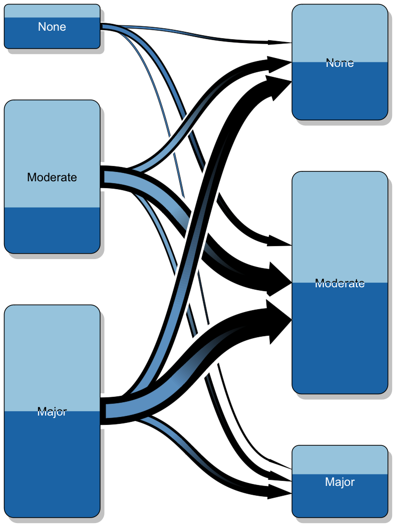
Ok, let's look at the output. As a nice example plot I use a
Yet, I don't think that SVG is always a good answer. The file size of an SVG file can grow quite quickly, if there are many points to be plotted. As an example check the difference in file size for two identical plots with 10,000 points.
Creating a SVG file with R could't be easier; e.g. use the
svg() function in the same way as png(). Next, make the file available online and embed it into your page. There are many ways to do this, in the example here I placed the file into a public GitHub repository.To embed the figure into my page I could use either the traditional
<img> tag, or perhaps better the <object> tag. Paul Murrell provides further details on his blog.With
<object> my code looks like this:<object data="https://rawgithub.com/mages/diesunddas/master/Blog/transitionPlot.svg" type="image/svg+xml" width="400"> </object>There is a little trick required to display a graphic file hosted on GitHub.
By default, when I look for the raw URL, GitHub will provide an address starting with
https://raw.githubusercontent.com/..., which needs to be replaced with https://rawgithub.com/....Ok, let's look at the output. As a nice example plot I use a
transitionPlot by Max Gordon, something I wanted to do for a long time.SVG output
PNG output
Conclusions
The SVG output is nice and crisp! Zoom in and the quality will not change. The PNG graphic on the other hand appears a little blurry on my screen and even the colours look washed out. Of course, the PNG output could be improved by fiddling with the parameters. But, after all it is a raster graphic.Yet, I don't think that SVG is always a good answer. The file size of an SVG file can grow quite quickly, if there are many points to be plotted. As an example check the difference in file size for two identical plots with 10,000 points.
x <- rnorm(10000)
png()
plot(x)
dev.off()
file.size("Rplot001.png")/1000
# [1] 118.071
svg()
plot(x)
dev.off()
file.size("Rplot001.svg")/1000
# [1] 3099.181
Update 10 Feb 2016
Or, is SVG the answer? Kenton pointed me towards the svglite package.library(svglite)
svglite(file = "Rplot001.svg")
plot(x)
dev.off()
file.size("Rplot001.svg")/1000
# [1] 973.619
gz <- function(in_path, out_path = tempfile()) {
out <- gzfile(out_path, "w")
writeLines(readLines(in_path), out)
close(out)
invisible(out_path)
}
file.size(gz("Rplot001.svg", "Rplot001.svgz")) / 1000
#> [1] 74.11R code
Session Info
R version 3.2.3 (2015-12-10)
Platform: x86_64-apple-darwin13.4.0 (64-bit)
Running under: OS X 10.11.3 (El Capitan)

locale:
[1] en_GB.UTF-8/en_GB.UTF-8/en_GB.UTF-8/C/en_GB.UTF-8/en_GB.UTF-8

attached base packages:
[1] grid      stats     graphics  grDevices utils     datasets
[7] methods   base

other attached packages:
[1] RColorBrewer_1.1-2 Gmisc_1.3          htmlTable_1.5
[4] Rcpp_0.12.3

loaded via a namespace (and not attached):
 [1] Formula_1.2-1       knitr_1.12.3
 [3] cluster_2.0.3       magrittr_1.5
 [5] splines_3.2.3       munsell_0.4.2
 [7] colorspace_1.2-6    lattice_0.20-33
 [9] stringr_1.0.0       plyr_1.8.3
[11] tools_3.2.3         nnet_7.3-12
[13] gtable_0.1.2        latticeExtra_0.6-26
[15] htmltools_0.3       digest_0.6.9
[17] forestplot_1.4      survival_2.38-3
[19] abind_1.4-3         gridExtra_2.0.0
[21] ggplot2_2.0.0       acepack_1.3-3.3
[23] rsconnect_0.3.79    rpart_4.1-10
[25] rmarkdown_0.9.2     stringi_1.0-1
[27] scales_0.3.0        Hmisc_3.17-1
[29] XML_3.98-1.3 foreign_0.8-66Flowing triangles
I have admired the work of the artist Bridget Riley for a long time. She is now in her eighties, but as it seems still very creative and productive. Some of her recent work combines simple triangles in fascinating compositions. The longer I look at them, the more patterns I recognise.
Yet, the actual painting can be explained easily, in a sense of a specification document to reproduce the pattern precisely. However, seeing the real print, as I had the chance at the London Art Fair last week, and a reproduction on the screen is incommensurable.
Having said that, I could not resist programming a figure that resembles the artwork labelled Bagatelle 2. Well, at least I can say that I learned more about

[2] P. Murrell. What's in a Name? . The R Journal, 4(2):5–12, dec 2012.
[3] P. Murrell and S. Potter. gridSVG: Export grid graphics as SVG. R package 1.5-0. 2015
Yet, the actual painting can be explained easily, in a sense of a specification document to reproduce the pattern precisely. However, seeing the real print, as I had the chance at the London Art Fair last week, and a reproduction on the screen is incommensurable.
Having said that, I could not resist programming a figure that resembles the artwork labelled Bagatelle 2. Well, at least I can say that I learned more about
grid [1], grid.path [2] and gridSVG [3] in R. R Code
References
[1] P. Murrell. R Graphics, Second Edition. CRC Press. 2011[2] P. Murrell. What's in a Name? . The R Journal, 4(2):5–12, dec 2012.
[3] P. Murrell and S. Potter. gridSVG: Export grid graphics as SVG. R package 1.5-0. 2015
Session Info
R version 3.2.3 (2015-12-10)
Platform: x86_64-apple-darwin13.4.0 (64-bit)
Running under: OS X 10.11.2 (El Capitan)

locale:
[1] en_GB.UTF-8/en_GB.UTF-8/en_GB.UTF-8/C/en_GB.UTF-8/en_GB.UTF-8

attached base packages:
[1] grid      stats     graphics  grDevices utils  datasets
[7] methods   base

other attached packages:
[1] gridSVG_1.5-0    data.table_1.9.6

loaded via a namespace (and not attached):
[1] tools_3.2.3   RJSONIO_1.3-0 chron_2.3-47  XML_3.98-1.3
Bridget Riley
,
grid
,
R
,
SVG


