Showing posts with label github. Show all posts
Showing posts with label github. Show all posts
Using SVG graphics in blog posts
My traditional work flow for embedding R graphics into a blog post has been via a PNG files that I upload online. However, when I created a 'simple' graphic with only basic curves and triangles for a recent post, I noticed that the PNG output didn't look as crisp as I expected it to be. So, eventually I used a SVG (scalable vector graphic) instead.
Creating a SVG file with R could't be easier; e.g. use the
To embed the figure into my page I could use either the traditional
With
There is a little trick required to display a graphic file hosted on GitHub.
By default, when I look for the raw URL, GitHub will provide an address starting with
Ok, let's look at the output. As a nice example plot I use a
Yet, I don't think that SVG is always a good answer. The file size of an SVG file can grow quite quickly, if there are many points to be plotted. As an example check the difference in file size for two identical plots with 10,000 points.
Creating a SVG file with R could't be easier; e.g. use the
svg() function in the same way as png(). Next, make the file available online and embed it into your page. There are many ways to do this, in the example here I placed the file into a public GitHub repository.To embed the figure into my page I could use either the traditional
<img> tag, or perhaps better the <object> tag. Paul Murrell provides further details on his blog.With
<object> my code looks like this:<object data="https://rawgithub.com/mages/diesunddas/master/Blog/transitionPlot.svg" type="image/svg+xml" width="400"> </object>There is a little trick required to display a graphic file hosted on GitHub.
By default, when I look for the raw URL, GitHub will provide an address starting with
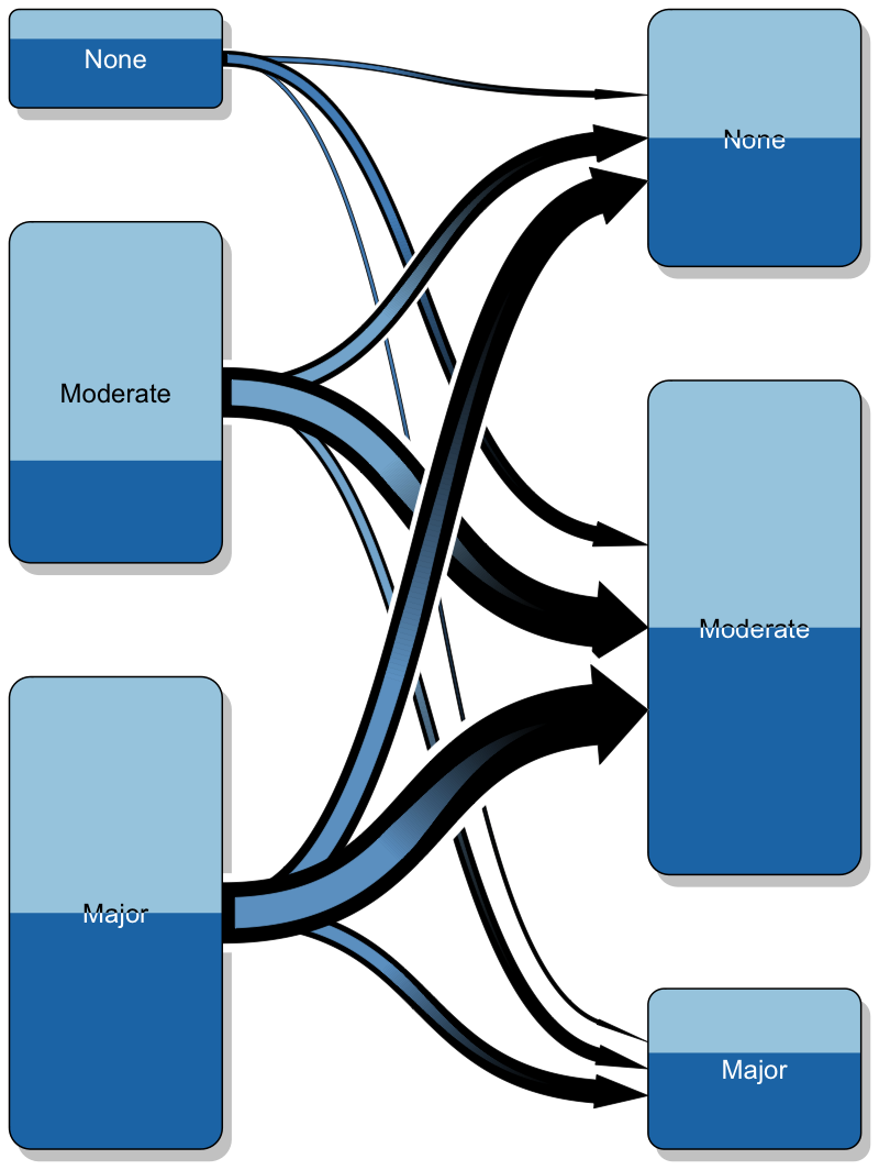
https://raw.githubusercontent.com/..., which needs to be replaced with https://rawgithub.com/....Ok, let's look at the output. As a nice example plot I use a
transitionPlot by Max Gordon, something I wanted to do for a long time.SVG output
PNG output
Conclusions
The SVG output is nice and crisp! Zoom in and the quality will not change. The PNG graphic on the other hand appears a little blurry on my screen and even the colours look washed out. Of course, the PNG output could be improved by fiddling with the parameters. But, after all it is a raster graphic.Yet, I don't think that SVG is always a good answer. The file size of an SVG file can grow quite quickly, if there are many points to be plotted. As an example check the difference in file size for two identical plots with 10,000 points.
x <- rnorm(10000)
png()
plot(x)
dev.off()
file.size("Rplot001.png")/1000
# [1] 118.071
svg()
plot(x)
dev.off()
file.size("Rplot001.svg")/1000
# [1] 3099.181
Update 10 Feb 2016
Or, is SVG the answer? Kenton pointed me towards the svglite package.library(svglite)
svglite(file = "Rplot001.svg")
plot(x)
dev.off()
file.size("Rplot001.svg")/1000
# [1] 973.619
gz <- function(in_path, out_path = tempfile()) {
out <- gzfile(out_path, "w")
writeLines(readLines(in_path), out)
close(out)
invisible(out_path)
}
file.size(gz("Rplot001.svg", "Rplot001.svgz")) / 1000
#> [1] 74.11R code
Session Info
R version 3.2.3 (2015-12-10)
Platform: x86_64-apple-darwin13.4.0 (64-bit)
Running under: OS X 10.11.3 (El Capitan)

locale:
[1] en_GB.UTF-8/en_GB.UTF-8/en_GB.UTF-8/C/en_GB.UTF-8/en_GB.UTF-8

attached base packages:
[1] grid      stats     graphics  grDevices utils     datasets
[7] methods   base

other attached packages:
[1] RColorBrewer_1.1-2 Gmisc_1.3          htmlTable_1.5
[4] Rcpp_0.12.3

loaded via a namespace (and not attached):
 [1] Formula_1.2-1       knitr_1.12.3
 [3] cluster_2.0.3       magrittr_1.5
 [5] splines_3.2.3       munsell_0.4.2
 [7] colorspace_1.2-6    lattice_0.20-33
 [9] stringr_1.0.0       plyr_1.8.3
[11] tools_3.2.3         nnet_7.3-12
[13] gtable_0.1.2        latticeExtra_0.6-26
[15] htmltools_0.3       digest_0.6.9
[17] forestplot_1.4      survival_2.38-3
[19] abind_1.4-3         gridExtra_2.0.0
[21] ggplot2_2.0.0       acepack_1.3-3.3
[23] rsconnect_0.3.79    rpart_4.1-10
[25] rmarkdown_0.9.2     stringi_1.0-1
[27] scales_0.3.0        Hmisc_3.17-1
[29] XML_3.98-1.3 foreign_0.8-66googleVis code development moved to GitHub
After nearly 4 years of developing googleVis on Google Code with SVN we decided to move to GitHub. The main reason was that Google stopped the facility of hosting pre-CRAN builds of the package for user testing. The
There are some exciting new features in the development version of 0.5.0-1 of googleVis, reflecting the enhanced Google Chart Tools API:
I will post about the new features and changes in the coming weeks. Please feel free to test the development version already. Visit our GitHub project page for installation instructions and further details.
For the impatient (you will require R >= 3.0.2):
devtools package on the other hand makes it really easy to install packages from source hosted on GitHub. Additionally, we hope that GitHub will make collaboration with others more effective. Thus, bookmark http://github.com/mages/googleVis. |
| Screen shot of some of the new features in googleVis 0.5.0-1. |
There are some exciting new features in the development version of 0.5.0-1 of googleVis, reflecting the enhanced Google Chart Tools API:
New Features
- New functions gvisSankey, gvisAnnotationChart, gvisHistogram, gvisCalendar and gvisTimeline to support the new Google charts of the same names (without 'gvis').
- New demo Trendlines showing how trend-lines can be added to Scatter-, Bar-, Column-, and Line Charts.
- New demo Roles showing how different column roles can be used in core charts to highlight data.
- New vignettes written in R Markdown showcasing googleVis examples and how the package works with knitr.
Changes
- The help files of gvis charts no longer show all their options, instead a link to the online Google API documentation is given.
- All googleVis output will be displayed in your default browser. In previous versions of googleVis output could also be displayed in the preview pane of RStudio. This feature is no longer available with the current version of RStudio, but is likely to be introduced again with the release of RStudio version 0.99 or higher.
I will post about the new features and changes in the coming weeks. Please feel free to test the development version already. Visit our GitHub project page for installation instructions and further details.
For the impatient (you will require R >= 3.0.2):
install.packages(c("devtools","RJSONIO", "knitr", "shiny", "httpuv"))
library(devtools)
install_github("mages/googleVis")Clone all your gists locally with R
I really like gists as a quick way to include more lengthly code snippets into my blog posts. However, I am not a git user as such, and so I was quite concerned when I noticed that all my gists on this blog had vanished after Christmas. I suppose this was a result of Github's downtime on December 22nd.
Thankfully an email to the support guys at Github resolved the issue within a few hours. Still, I thought it might be a good idea to download my gists locally.
I can see all my gists as a JSON file online here:
Thus, I downloaded the file and thanks to the RJSONIO package I was able to clone all my gists locally with a few lines of R:
Thankfully an email to the support guys at Github resolved the issue within a few hours. Still, I thought it might be a good idea to download my gists locally.
I can see all my gists as a JSON file online here:
https://api.github.com/users/MYUSERLOGIN/gistsThus, I downloaded the file and thanks to the RJSONIO package I was able to clone all my gists locally with a few lines of R:


